Description
The following case study is realized on a block model of a massive polimetalic deposit with copper as the main mineral. The aim is to compare the traditional scheduling methodology of nested pits and the direct block scheduling using the computational software DOPPLER (Delphos Open Pit Planner), developed at the Mine Planning Lab DELPHOS.
Model Definition
Name: definitivo2_bme
Number of blocks: 74.849
Dimensions: 20 x 20 x 15
Coordinates range: x = 26.799.98 to 29.519,98
y = 80.810,17 to 82.950,17
z = 3.992,50 to 4.667,50
Model variables: Cobre, Molibdeno, Oro, Plata, Recuperación Metalurgica, Recuperación Metalúrigica del Molibdeno, Densidad
Additionally, it was added columns from the previous ones, according to model parameters and requirements.
Block Model Visualization
As it can be seen from the image below, the greatest grades concentrate at the bottom of the deposit.

Isometric View

Frontal View Plan view
The shape of the model is explained by a preexisting pit.
Grade-Tonnage Graph
From the image below one can see that the sensibility of the ore tonnage by the grade is high.
Grade Distribution
The vast majority of the blocks are associated with low grades.

Economic parameters
It was executed 3 cases of valuation, which vary by the copper price.
| Valuation |
Copper price [USD/lb] |
| A | 2.0 |
| B | 2.5 |
| C | 1.5 |
Scheduling by Nested-Pits
Based on the pseudo-flow algorithm, the Final Pit and its Nested-Pits were determined, upon which it was done the traditional scheduling by phase-bench, considering specific parameters for the Project. From a parametric price multiplication, the “Revenue Factor”, different envelopes were generated (nested pits), on which pushbacks or “phase-candidates” that can be used as a guide to the scheduling were chosen.
Problem Description
It was executed three valuations for the main economic element, Copper. For each one of them, Final Pit and Nested Pits are determined. The conditions on which the analysis were done are as it follows:
Two destinations: Processing Plant and Waste Dump
Capacity restrictions: Mining and Processing
No blending restrictions are considered.
Final Pit

Nested Pits

Best and Worst Case
To speed up development work, case B was chosen for further analysis, so from now on the focus will be case B.
Best Case - Valuation B
Scheduling by "Pit and Bench" – Case B.
Total Tonnage: 70 [Mton]


Isometric View
Worst Case - Valuation B
Scheduling by "Bench" - Case B.
Total Tonnage: 70 [Mton]


Isometric View
Direct Block Scheduling (DBS)
The Direct Block Scheduling is an alternative way which emphasis the temporality of the problem and the opportunity cost, searching to solve since the beggining the problem of when is more convenient to extract a block and what destination should it take (processing plant or waste dump). Traditionally, this methodology is based on big linear programming models.
The software Doppler provides the Direct Block Scheduling – BOS2M. Next it is possible to see the input parameters:
Mine Capacity: 70 [Mt]
Plant Capacity: 50 [Mt]
Horizon: 10 periods


Isometric View
Phase-Bench-Destination Scheduling by UDESS
It’s done a scheduling by phase-bench-destination on the software UDESS.
The original block model has a default tonnage column, which was used to do the scheduling.
For each block in the block model it is predefined a destination – plant or waste dump – according to which of them provide the greatest profit.
For the block value calculation the following tecnical-economical parameters are applied: Copper Price: 2.5 [USD/t], Mine Cost: 2.5 [USD/t], Plant Cost: 10 [USD/t], Refining Cost: 0.5 [USD/lb].
Afterwards, it is obtained the total tonnage, profit and copper fines for each phase, bench and destination.
The objective function is to maximize NPV with a discount rate of 10%.
The constraints are the mine capacity of 70 [Mt/year] and a processing capacity of 20 [Mt/año]. The maximum and minimum difference between consecutive phases are 4 and 1 benches, respectively.
The NPV (10%) obtained is de 3 886 [MUSD]. The average grade of recovered copper fine is 0.87 %. Total recovered fine is 2468 [kt]. Waste tonnage and ore tonnage is 347 and 285 [Mt]. Mine life of 10 years.
The following parameters are applied:
Minimum difference between benches: 1
Maximum difference between benches: 4
Mine Capacity: 70 Mt/year
Plant Capacity: 50 Mt/year
Discount Rate: 10%
Valuation B

Comparision
Considering a discount rate of 10%, the differences are significant.
NPV Toposort: 6 472 929 122 USD
NPV Full MIP: 6 487 514 853 USD
NPV UDESS: 3 886 000 000 USD
Conclusions
For this exemple, two of the optmization methods available in Doppler were used, Toposort and Full MIP. It is worth mentioning that the execution time for each one varies depending on the constraints applied.
As it can be seen in the previous item, NPV provided by Full MIP is greater than the one provided by Toposort.
NPV (10%) obtained algorithms for the direct scheduling block (Toposort and Full MIP) is similar.
Otherwise, the NPV obtained by direct scheduling algorithms block is considerably higher than obtained by prior definition phase. This happens because the direct block scheduling can select any blocks within a bench, while the phase-based scheduling, you must remove all waste and then start extraction of ore.
Also, the extraction is more restrictive in the case based in phase scheduling, since it does not support the deepening of many benchs as possible if direct block scheduling.
Thus, the scheduling based in phase is more feasible to carry out that direct the scheduling block. However, the definition phase to carry out this scheduling is performed using criteria scheduler turn.
Efforts should be made to the definition of phases that do not depend on the judgment of shift planner.
Description
This example compares the results obtained from the traditional Nested Pit approach and the Direct Block Scheduling methodology for production scheduling in open pit mine planning.
Scheduling using Nested Pits
Using the Lerchs & Grossmann algorithm on several block model valorizations scaled by the revenue factor. From the generated nested pits, pushbacks are selected, which are useful as a design guide. Then, this pushbacks are sheduled for extraction.
Scheduling using Direct Block Scheduling
This is an alternative approach where the emphasis is focused on time and opportunity cost,looking for a solution from the moment that is better to extract the block and what is the better choice of processing (including the waste option). This methodology is based on linear programming models.
Block Model
| Name | MDB RAJO |
| Number of blocks | 151.898 |
| Dimensions | 5 x 5 x 5 |
| Coordinates range |
X=214.961,125 - 215.251,125 Y=8.080.666,5 - 8.081.201,5 Z=247,5 - 422,5 |
|
Model columns |
zone, au, ag, cu, denisty |
| Comments | Tonnage column was added |
Model Visualization
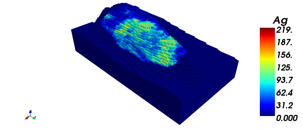
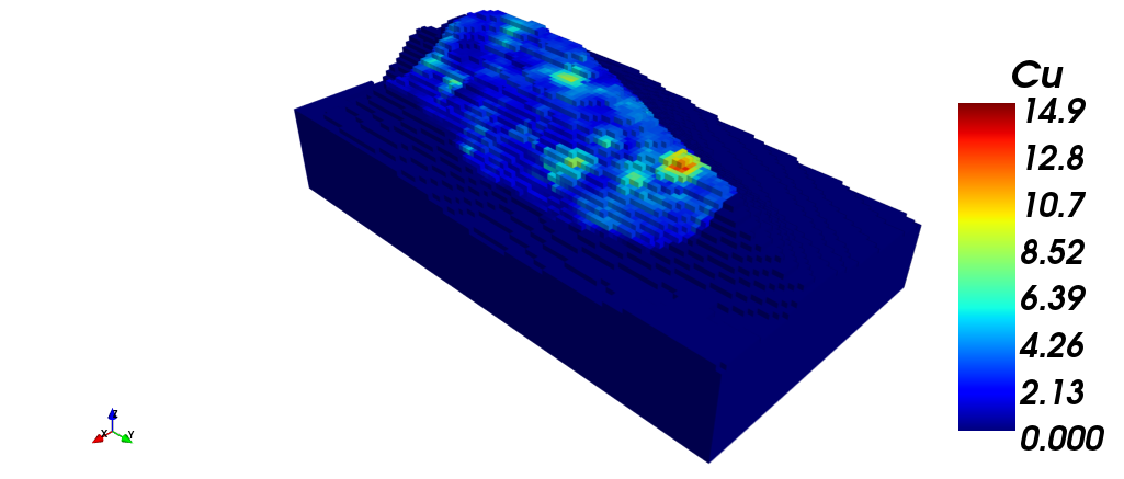
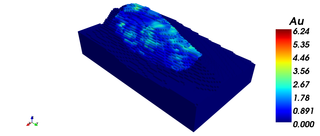
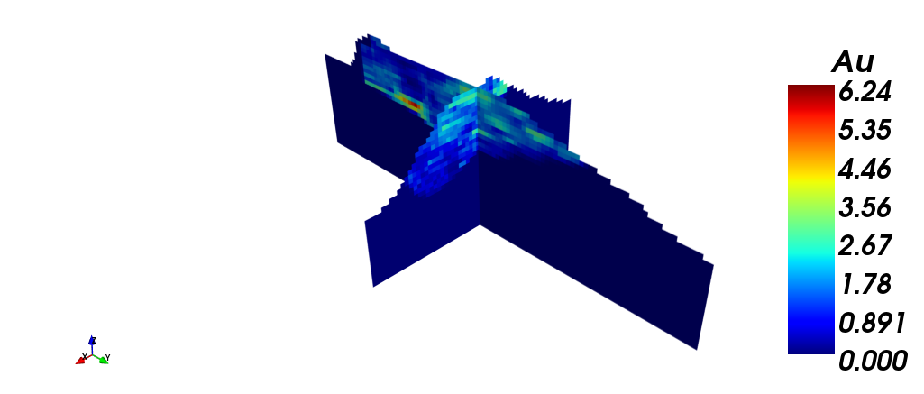
The following images show the block model with: (i) Silver grade; (ii) Copper grade; (iii) Gold grade. Finally, a section view is shown, filtered by gold grade.
|
|
 |
| (i) | (ii) |
 |
 |
| (iii) | (iv) |
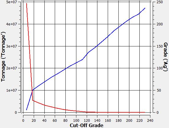
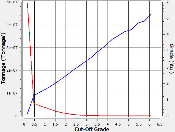
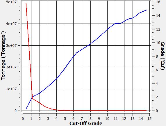
Tonnage-grade curves
Three curves are shown, one for each metal in the block model: (i) silver, (ii) gold, (iii) copper.
 |
 |
 |
| (i) | (ii) | (iii) |
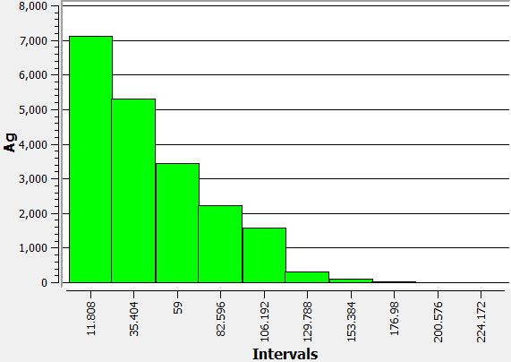
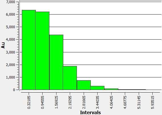
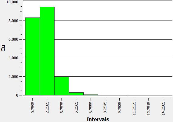
Grade distribution
For each metal in the block model, the grade distribution is shown: (i) silver, (ii) gold, (iii) copper.
|
|
 |
 |
| (i) | (ii) | (iii) |
Final Pit
Block valuation and slope angles
Valorization data:
1) Metal prices: Ag = 16 [USD/oz]; Au = 1.100 [USD/oz]; Cu = 2,0 [USD/lb]
2) Sell cost: Ag = 1,6 [USD/oz]; Au = 100 [USD/oz]; Cu = 0,3 [USD/lb]
3) Processing cost: Ag = 8,0 [USD/Ton]; Au = 8,2 [USD/Ton]; Cu = 8,0 [USD/Ton]
4) Metallurgical recovery: Ag = 0,77; Au = 0,76; Cu = 0,85
5) Mine cost: 1,5 [USD/Ton]
Slope angle data:
1) 48° (global)
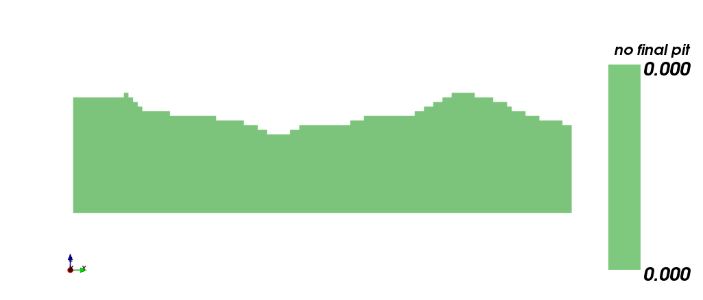
Final pit visualization
The following images show the final pit obtained from the block model and the valorization parameteres above. (i) isometric view, (ii) section view.
 |
 |
| (i) | (ii) |
Nested Pits
Block valuation and slope angles
The same parameters were used, but using some revenue factors for each final pit, nested pits are obtained. The revenue factor family selected goes from 0 to 1, using a 0.05 step.
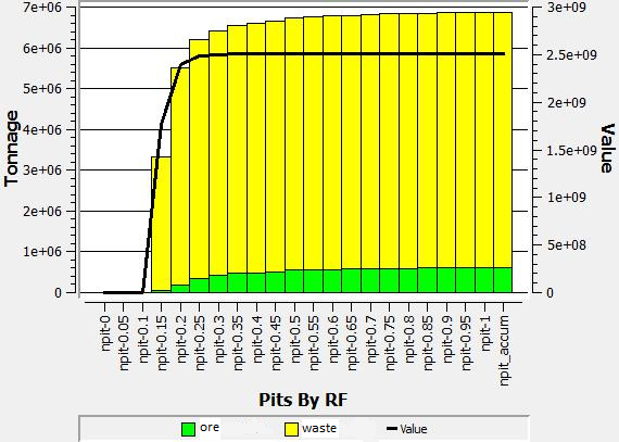
Pit By Pit Chart
Nested pits visualization
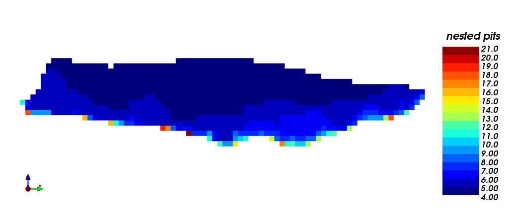
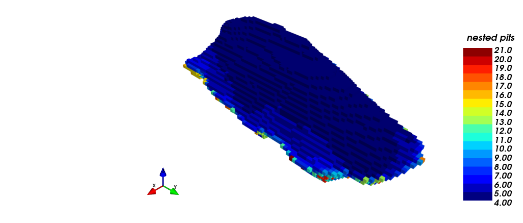
In the following pictures, a family of nested pits are shown, which were obtained from the revenue factors: (i) isometric view of the pits, inside of the economic envelope, meanwhile (ii) shows a section view. The first pit with positive economic value is the one with revenue factor 0.15.
 |
|
| (i) | (ii) |
Best & Worst Case
Production plan best case
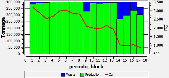
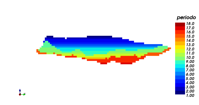
In this case, the extraction is made following the order of the nested pits. A limit of extracted tonnage of 400.000 [Ton] was set, and a 18 anual periods horizon was obtained. It should be noted that the maximum production was reached in several periods, leaving for the final periods the greatest waste portions. (i) production plan, (ii) scheduling section view, both using the best case strategy, pit by pit.
 |
 |
| (i) | (ii) |
Production plan worst case
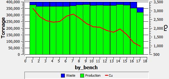
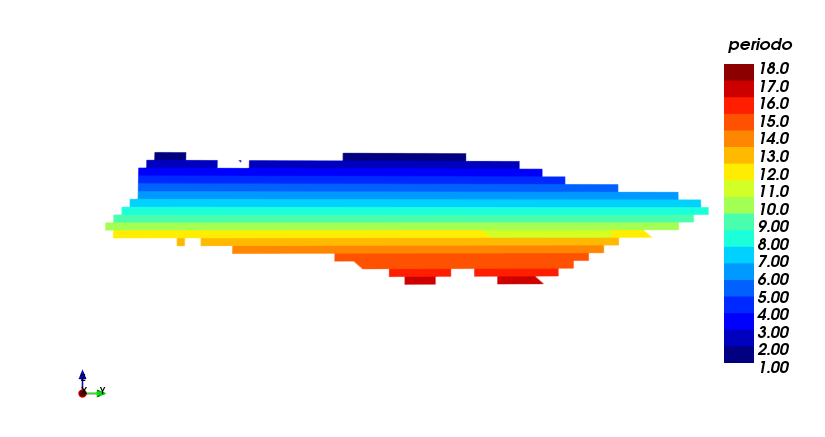
In this case, the extraction is made following the order bench by bench. Same as before, a limit of extracted tonnage of 400.000 [Ton] was set, and a 18 anual periods horizon was obtained. It should be noted that both production and waste are well distributed along the project horizon. Nevertheless, the are not greater differences besides the one mentioned before. (i) production plan, (ii) scheduling section view, both using the worst case strategy, bench by bench.
 |
 |
| (i) | (ii) |
Direct Block Scheduling
In this section, a direct block scheduling will be applied. For its resolution, two strategies will be used: (i) Sliding time windows heuristic, in which the problem is solved in an incremental manner using a period window (lower than the horizon) and setting this window as a complete or partial solution and (ii) Toposort heuristic, in which the continuous relaxation of the problem is exploded and defines the expected time to do a scheduling using the order given by the expected time and production capacities.
Input Parameters
Number of periods: 18
Discount rate: 10%
Slope angle: 48° (global)
Valorization according to destination:
- Value to plant: each block is valued as if its final destination is the processing plant
- Value to dump: each block is valued as if its final destination is the dump
Capacities by period:
- Mine: 400.000 [ton]
- Plant: 350.000 [ton]
Choosing optimal block destinations
Sliding time windows heuristic results (window: 1, step: 1)
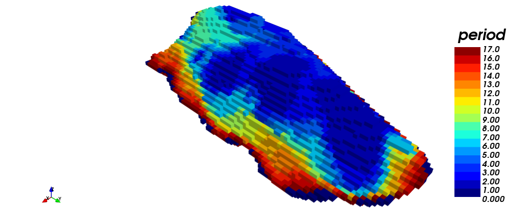
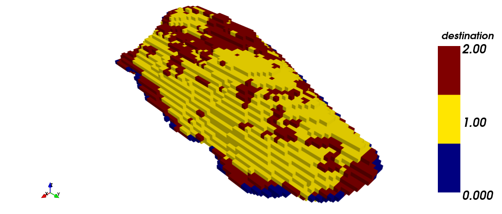
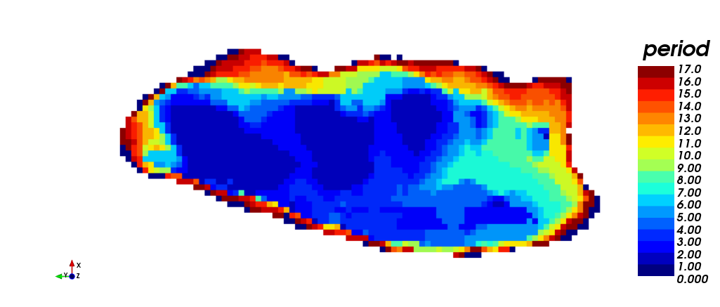
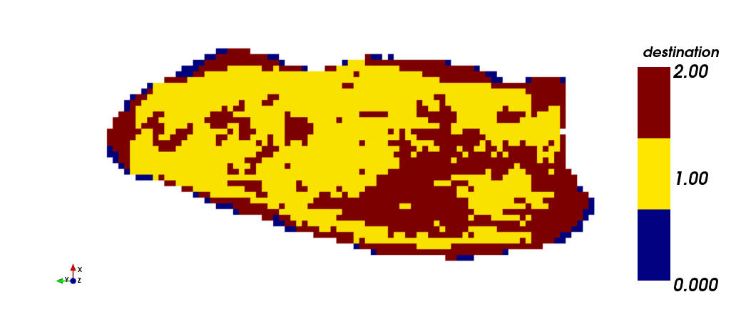
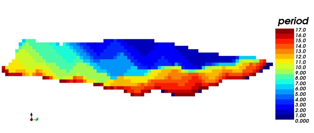
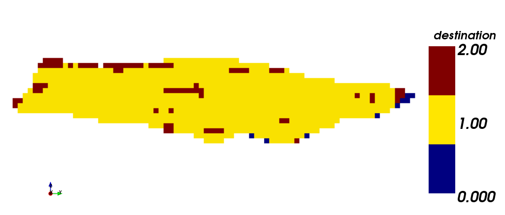
In the following pictures the different views of the scheduling process through STW are shown. (i) isometric view, (iii) plant view and (v) section view. It should be noted that 17 periods were required for production scheduling. On the other hand, the scheduling according to destination is shown. (ii) isometric view, (iv) plant view and (vi) section view. In yellow (1) is shown the material sent to process plant, in red (2) the material sent to dump, and in blue (0) the material that has never been extracted.
 |
 |
| (i) | (ii) |
 |
 |
| (iii) | (iv) |
 |
 |
| (v) | (vi) |
Production plan using STW heuristic
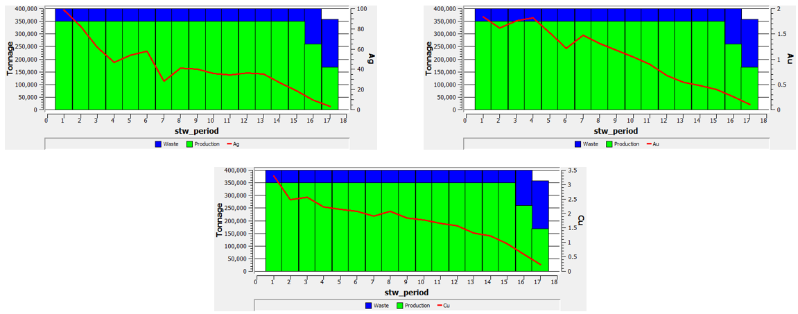
The production plan (mineral and waste) and the mean grade for each metal are shown in the following images.
Toposort heuristic results
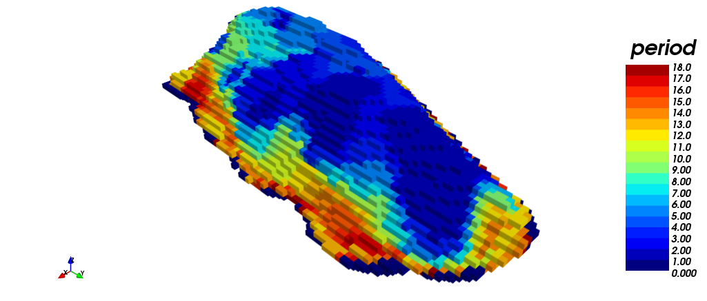
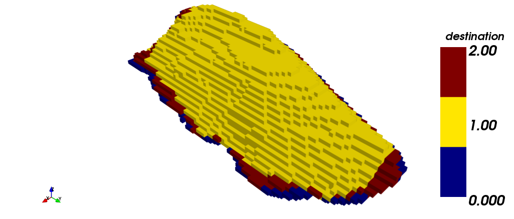
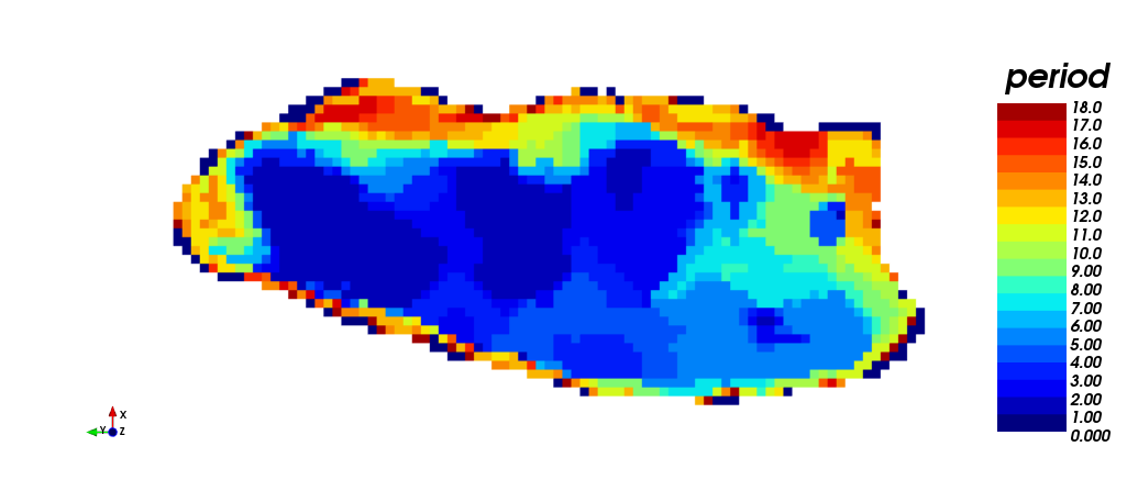
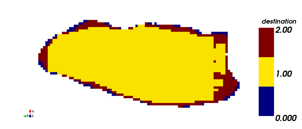
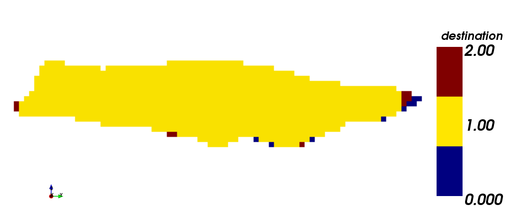
The images below show different views of the scheduling obtained through the toposort heuristic. (i) isometric view, (iii) plant view and (v) section view. It should be noted that this case required the 18 periods for production scheduling, unlike STW heuristic. On the other hand, the scheduling according to destination is shown. (ii) isometric view, (iv) plant view and (vi) section view. In yellow (1) is shown the material sent to process plant, in red (2) the material sent to dump, and in blue (0) the material that has never been extracted. The difference between both STW heuristic and Toposort heurisctic should be noted: many of the blocks that STW sent to dump, Toposort classified them as mineral to process plant.
 |
 |
| (i) | (ii) |
 |
 |
| (iii) | (iv) |
 |
 |
| (v) | (vi) |
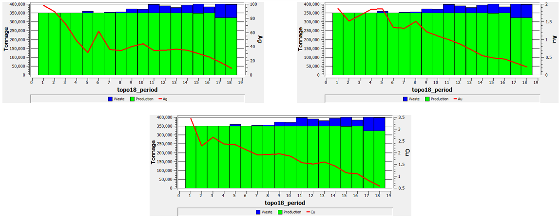
Production plan using toposort heuristic
The production plan (mineral and waste) and the mean grade for each metal are shown in the following images.
Comparison and results
Considering the results obtained by both heuristics, it is clear that toposort made the schedule in 18 periods, as was required, meanwhile stw heuristic did the same in 17 periods. Looking at the production plans, topo could delayed the waste entrance in the first periods, classifying as mineral all the material extracyed between the periods 1 and 4, and also the 6th period, and from there extracting gradually the waste material completing the mine capacity in the final periods.
Meanwhile, STW made an homogeneous extraction, saturating both mine and plant capacities in most of the periods (except 16 and 17).
The myopic characteristic of STW doesnt let the heuristic to make decisions for later periods, instead of that, the heuristic make the best decisions possible for each period. On the other hand, topo is capable to make a global decision from the information obtained from the continuous solution of the original problem, and for this reasons is considered a robust decision, that is to say, to make a decision about a particular period, the heuristic looks what happen in later periods and then makes the decision.
In terms of cumulative present value (NPV), the topo strategy shows a greater NPV than the STW strategy (0.23% higher).
NPV STW : 1.386 [MUSD]
NPV TOPO : 1.390 [MUSD]
In general , this knd of strategies cannot ensure to find an optimal solution for the scheduling problem, but they are a good alternative considering real problems with great dimensions (number of blocks, periods and destinations), where the idea to solve directly is practicly
BLOCK MODELS
The block model size for this work has 4.320.287 blocks. In this model the principal variables are the size in the three principal direction(X, Y, Z), lithology, density, 25 conditional simulation of for copper and average copper grade.
With the variables density and the size of each block, the tonnage of each block can be calculated. For this work only the average of the 25 simulations and the first conditional simulation are used.
BLOCK MODEL VIEWS
The next images show a few views of the copper in the 2 cases that are considered.
Image of Block model showing the average for the copper grades from the conditional simualtions
Image of Block model showing the first conditional of copper grade
From the images presented befored it can be see that the variability of copper grade for the first conditional simulation is higher than the case made with the mean. If we look the scale of the images for the different cases, it´s easy to see that the máximum of the conditional simulation goes to 7% aprox. and the scenario constructed from the mean of all the conditional simulation only reaches to the 3%.
TONNAGE V/S GRADE CHART AND HISTOGRAMS OF COPPER GRADE DISTRIBUTION
The Tonnage-Grade charts are presented below.
Tonnage-Grade chart for the case of the average from all conditionals simulations
Tonnage-Grade chart for the first conditional simulation scenario
VALUATION INPUTS AND SLOPE ANGLES
The inputs that are used to do the valuation and the optimization process of the block model, it can be see in the next table.
| Cu price [US$/lb] | 1.5 |
| Costo Mine Cost [US$/t] | 3 |
| Costo Plant Cost [US$/t] | 13 |
| Recovery [%] | 85 |
| Fundition and Refination Cost [US$/lb] | 0.65 |
| Slope Angle [°] | 45 |
| Precedence levels [N°] | 6 (Z Diff 75) |
Economic
NESTED PIT AND SELECTION OF THE FINAL PIT
In generation of the production plan for the best case and worst case, we restrict the material movement per year to 200 millions, and a discont rate of 10%.
The result of the Best case production plan are presented next.
Production plan for the best case scenario of the average from all conditionals simulations
Production plan for the best case scenario for the first conditional simulation scenario
| |
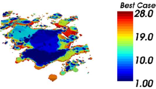 |
Views of the production plan for the best cases escenario, for the both cases, Mean case (Right) and first conditional simualtion (left).
The result of the Worst case production plan are presented next
Production plan for the worst case scenario of the average from all conditionals simulations
Production plan for the best case scenario for the first conditional simulation scenario
|
|
|
Views of the production plan for the best cases escenario, for the both cases, Mean case (Right) and first conditional simualtion (left).
As we can se from the production plan charts for the best case and worst case, the value of the plan increase year by year. En the last periods of the plans, this increment it´s less important because the effect of the discount rate.
PRODUCTION PLANS BY DIRECT BLOCK SCHEDULLING
In the construction of this production plan we use the same restriction of material movment of the mine, and we add a restriction to the capacity of the process plant of 95 millions. Finally the same discount rate than the previous cases.
A few views of the optimization results are presented next.
|
|
|
The average from all conditionals simulations (Left) and the first conditional simulation scenario (Right)
As can be see in the previous images, the production plan of the average scenario it{s softer tha the result with the first conditional simualtion.
Production plan for the the average from all conditionals scenario
Production plan for the first conditional simulation scenario
We can see from the charts that the feeding to the processing plant it always at th máximum capacity. But the movement of wast from the mine presents a high variabilty between periods. Finally the Cu grade even though has a lot of variability between periods, in general has a decrecent tendence
The net present value for each scenario are presented in the table below.
| Scenario | NPV |
| [MUS$] | |
| Average | 3,489 |
| Conditional Simulation | 2,574 |
NPV for each scenario
As we can see from the table, the NPV of the average scenario it´s 45% aproc. higher than the Conditional simulation scenario.


