BLOCK MODELS
The block model size for this work has 4.320.287 blocks. In this model the principal variables are the size in the three principal direction(X, Y, Z), lithology, density, 25 conditional simulation of for copper and average copper grade.
With the variables density and the size of each block, the tonnage of each block can be calculated. For this work only the average of the 25 simulations and the first conditional simulation are used.
BLOCK MODEL VIEWS
The next images show a few views of the copper in the 2 cases that are considered.
Image of Block model showing the average for the copper grades from the conditional simualtions
Image of Block model showing the first conditional of copper grade
From the images presented befored it can be see that the variability of copper grade for the first conditional simulation is higher than the case made with the mean. If we look the scale of the images for the different cases, it´s easy to see that the máximum of the conditional simulation goes to 7% aprox. and the scenario constructed from the mean of all the conditional simulation only reaches to the 3%.
TONNAGE V/S GRADE CHART AND HISTOGRAMS OF COPPER GRADE DISTRIBUTION
The Tonnage-Grade charts are presented below.
Tonnage-Grade chart for the case of the average from all conditionals simulations
Tonnage-Grade chart for the first conditional simulation scenario
VALUATION INPUTS AND SLOPE ANGLES
The inputs that are used to do the valuation and the optimization process of the block model, it can be see in the next table.
| Cu price [US$/lb] | 1.5 |
| Costo Mine Cost [US$/t] | 3 |
| Costo Plant Cost [US$/t] | 13 |
| Recovery [%] | 85 |
| Fundition and Refination Cost [US$/lb] | 0.65 |
| Slope Angle [°] | 45 |
| Precedence levels [N°] | 6 (Z Diff 75) |
Economic
NESTED PIT AND SELECTION OF THE FINAL PIT
In generation of the production plan for the best case and worst case, we restrict the material movement per year to 200 millions, and a discont rate of 10%.
The result of the Best case production plan are presented next.
Production plan for the best case scenario of the average from all conditionals simulations
Production plan for the best case scenario for the first conditional simulation scenario
| |
 |
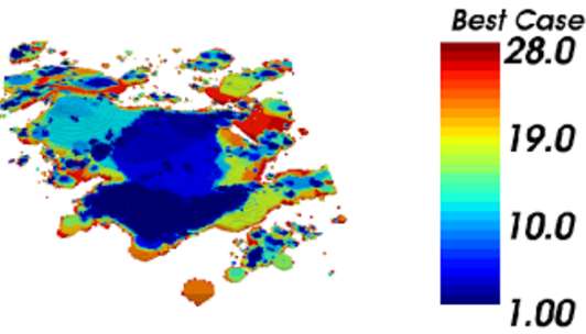
Views of the production plan for the best cases escenario, for the both cases, Mean case (Right) and first conditional simualtion (left).
The result of the Worst case production plan are presented next
Production plan for the worst case scenario of the average from all conditionals simulations
Production plan for the best case scenario for the first conditional simulation scenario
|
|
|
Views of the production plan for the best cases escenario, for the both cases, Mean case (Right) and first conditional simualtion (left).
As we can se from the production plan charts for the best case and worst case, the value of the plan increase year by year. En the last periods of the plans, this increment it´s less important because the effect of the discount rate.
PRODUCTION PLANS BY DIRECT BLOCK SCHEDULLING
In the construction of this production plan we use the same restriction of material movment of the mine, and we add a restriction to the capacity of the process plant of 95 millions. Finally the same discount rate than the previous cases.
A few views of the optimization results are presented next.
|
|
|
The average from all conditionals simulations (Left) and the first conditional simulation scenario (Right)
As can be see in the previous images, the production plan of the average scenario it{s softer tha the result with the first conditional simualtion.
Production plan for the the average from all conditionals scenario
Production plan for the first conditional simulation scenario
We can see from the charts that the feeding to the processing plant it always at th máximum capacity. But the movement of wast from the mine presents a high variabilty between periods. Finally the Cu grade even though has a lot of variability between periods, in general has a decrecent tendence
The net present value for each scenario are presented in the table below.
| Scenario | NPV |
| [MUS$] | |
| Average | 3,489 |
| Conditional Simulation | 2,574 |
NPV for each scenario
As we can see from the table, the NPV of the average scenario it´s 45% aproc. higher than the Conditional simulation scenario.


