Description

This example compares the results obtained from the traditional Nested Pit approach and the Direct Block Scheduling methodology for production scheduling in open pit mine planning.

Scheduling using Nested Pits

Using the Lerchs & Grossmann algorithm on several block model valorizations scaled by the revenue factor. From the generated nested pits, pushbacks are selected, which are useful as a design guide. Then, this pushbacks are sheduled for extraction.

Scheduling using Direct Block Scheduling

This is an alternative approach where the emphasis is focused on time and opportunity cost,looking for a solution from the moment that is better to extract the block and what is the better choice of processing (including the waste option). This methodology is based on linear programming models.

Block Model

Name	MDB RAJO
Number of blocks	151.898
Dimensions	5 x 5 x 5
Coordinates range	X=214.961,125 - 215.251,125 Y=8.080.666,5 - 8.081.201,5 Z=247,5 - 422,5
Model columns	zone, au, ag, cu, denisty
Comments	Tonnage column was added

 

Model Visualization

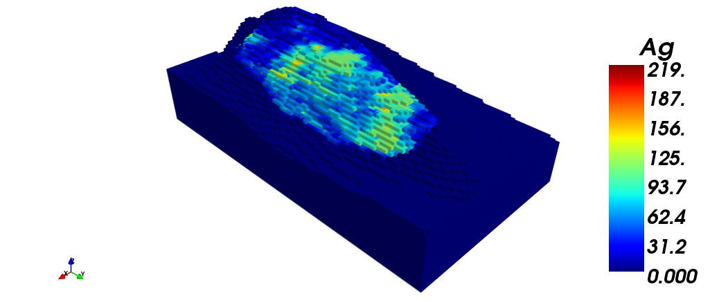
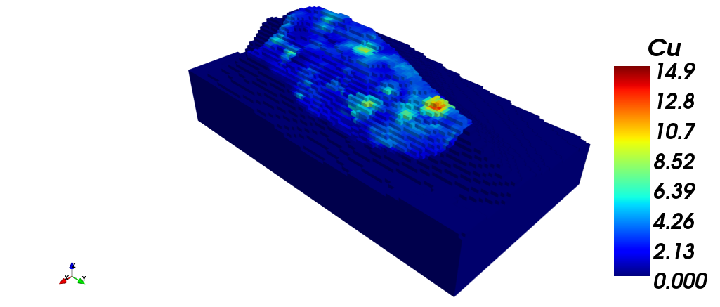
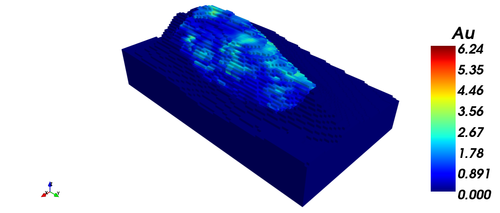
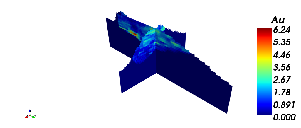
The following images show the block model with: (i) Silver grade; (ii) Copper grade; (iii) Gold grade. Finally, a section view is shown, filtered by gold grade.

(i)	(ii)
(iii)	(iv)

Tonnage-grade curves

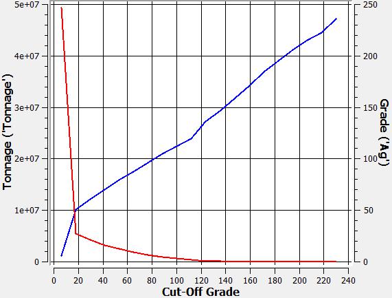
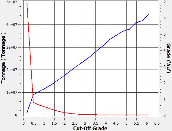
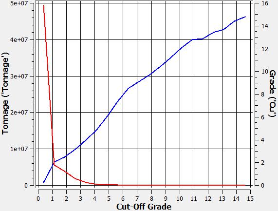
Three curves are shown, one for each metal in the block model: (i) silver, (ii) gold, (iii) copper.

(i)	(ii)	(iii)

Grade distribution

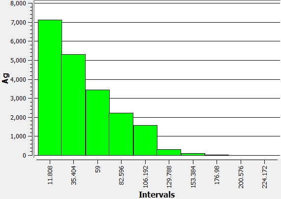
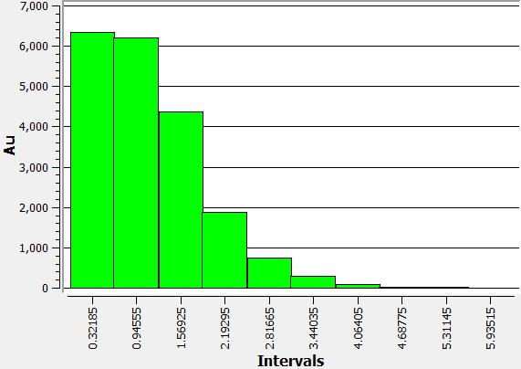
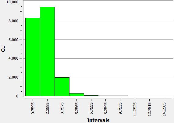
For each metal in the block model, the grade distribution is shown: (i) silver, (ii) gold, (iii) copper.

(i)	(ii)	(iii)

 

Final Pit

Block valuation and slope angles

Valorization data:

1) Metal prices: Ag = 16 [USD/oz]; Au = 1.100 [USD/oz]; Cu = 2,0 [USD/lb]
2) Sell cost: Ag = 1,6 [USD/oz]; Au = 100 [USD/oz]; Cu = 0,3 [USD/lb]
3) Processing cost: Ag = 8,0 [USD/Ton]; Au = 8,2 [USD/Ton]; Cu = 8,0 [USD/Ton]
4) Metallurgical recovery: Ag = 0,77; Au = 0,76; Cu = 0,85
5) Mine cost: 1,5 [USD/Ton]

Slope angle data:

1) 48° (global)

Final pit visualization

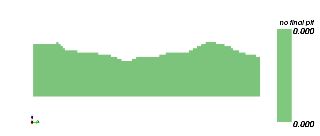
The following images show the final pit obtained from the block model and the valorization parameteres above. (i) isometric view, (ii) section view.

(i)	(ii)

 

Nested Pits

Block valuation and slope angles

The same parameters were used, but using some revenue factors for each final pit, nested pits are obtained. The revenue factor family selected goes from 0 to 1, using a 0.05 step.

Pit By Pit Chart

 

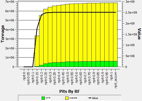
Nested pits visualization

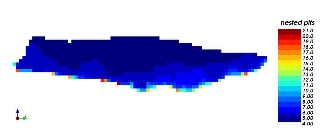
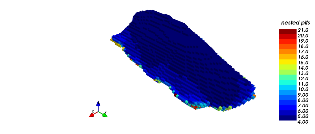
In the following pictures, a family of nested pits are shown, which were obtained from the revenue factors: (i) isometric view of the pits, inside of the economic envelope, meanwhile (ii) shows a section view. The first pit with positive economic value is the one with revenue factor 0.15.

(i)	(ii)

Best & Worst Case

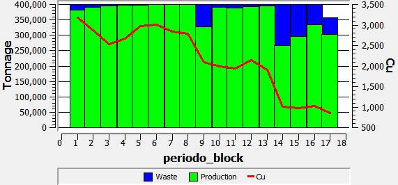
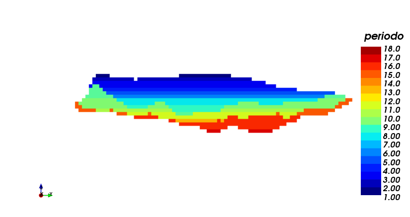
Production plan best case

In this case, the extraction is made following the order of the nested pits. A limit of extracted tonnage of 400.000 [Ton] was set, and a 18 anual periods horizon was obtained. It should be noted that the maximum production was reached in several periods, leaving for the final periods the greatest waste portions. (i) production plan, (ii) scheduling section view, both using the best case strategy, pit by pit.

(i)	(ii)

Production plan worst case

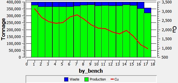
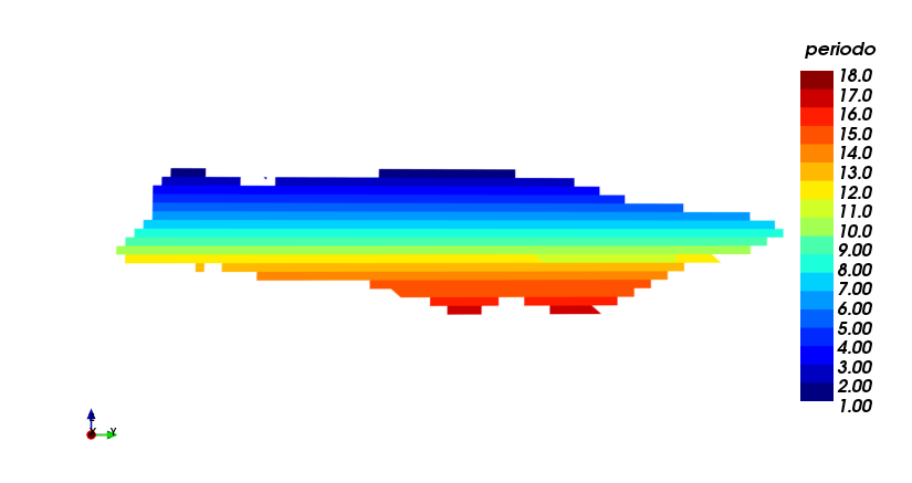
In this case, the extraction is made following the order bench by bench. Same as before, a limit of extracted tonnage of 400.000 [Ton] was set, and a 18 anual periods horizon was obtained. It should be noted that both production and waste are well distributed along the project horizon. Nevertheless, the are not greater differences besides the one mentioned before. (i) production plan, (ii) scheduling section view, both using the worst case strategy, bench by bench.

(i)	(ii)

Direct Block Scheduling

In this section, a direct block scheduling will be applied. For its resolution, two strategies will be used: (i) Sliding time windows heuristic, in which the problem is solved in an incremental manner using a period window (lower than the horizon) and setting this window as a complete or partial solution and (ii) Toposort heuristic, in which the continuous relaxation of the problem is exploded and defines the expected time to do a scheduling using the order given by the expected time and production capacities.

Input Parameters

Number of periods: 18
Discount rate: 10%
Slope angle: 48° (global)
Valorization according to destination:
- Value to plant: each block is valued as if its final destination is the processing plant
- Value to dump: each block is valued as if its final destination is the dump
Capacities by period:
- Mine: 400.000 [ton]
- Plant: 350.000 [ton]

Choosing optimal block destinations

Sliding time windows heuristic results (window: 1, step: 1)

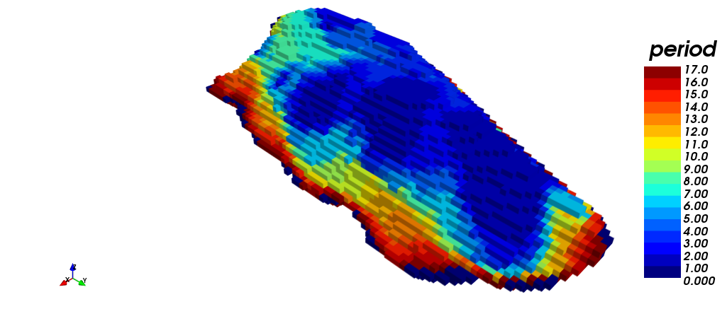
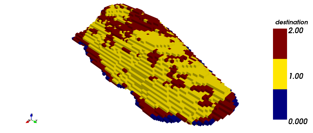
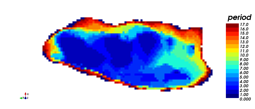
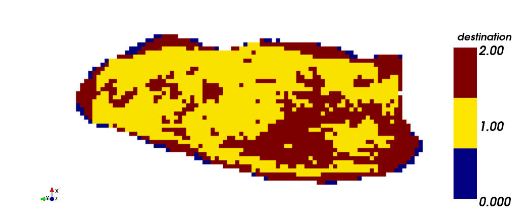
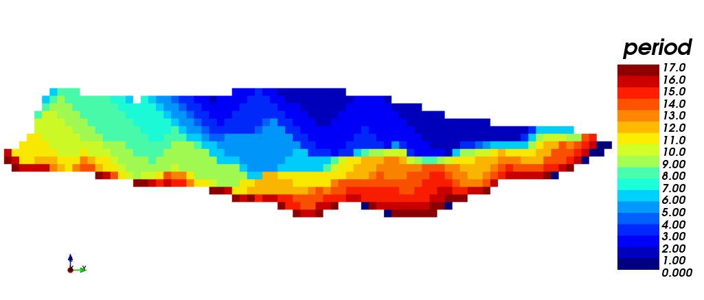
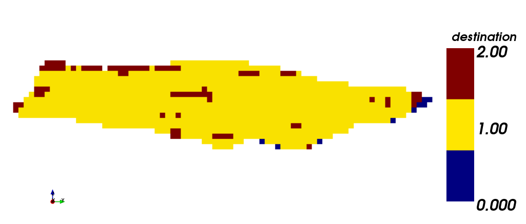
In the following pictures the different views of the scheduling process through STW are shown. (i) isometric view, (iii) plant view and (v) section view. It should be noted that 17 periods were required for production scheduling. On the other hand, the scheduling according to destination is shown. (ii) isometric view, (iv) plant view and (vi) section view. In yellow (1) is shown the material sent to process plant, in red (2) the material sent to dump, and in blue (0) the material that has never been extracted.

(i)	(ii)
(iii)	(iv)
(v)	(vi)

Production plan using STW heuristic

The production plan (mineral and waste) and the mean grade for each metal are shown in the following images.

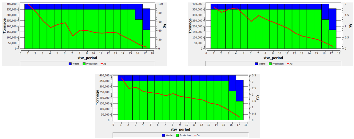
Toposort heuristic results

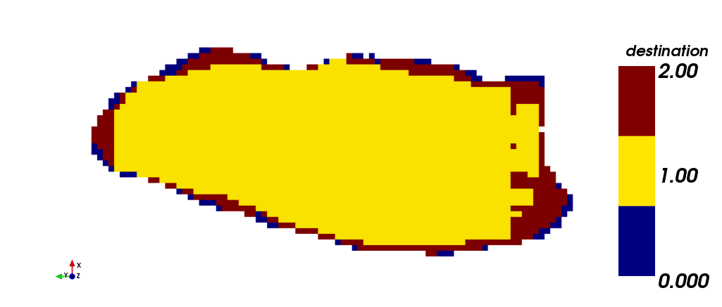
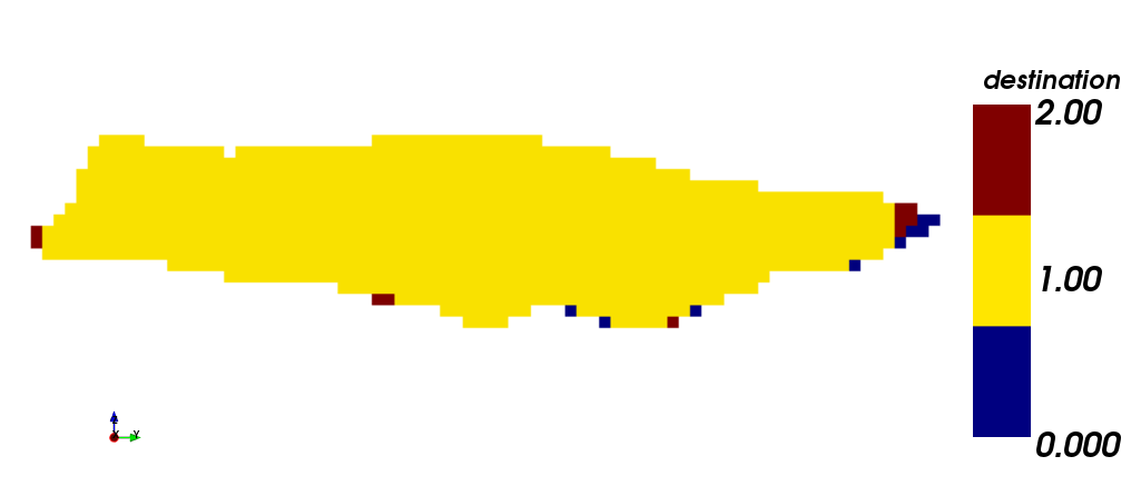
The images below show different views of the scheduling obtained through the toposort heuristic. (i) isometric view, (iii) plant view and (v) section view. It should be noted that this case required the 18 periods for production scheduling, unlike STW heuristic. On the other hand, the scheduling according to destination is shown. (ii) isometric view, (iv) plant view and (vi) section view. In yellow (1) is shown the material sent to process plant, in red (2) the material sent to dump, and in blue (0) the material that has never been extracted. The difference between both STW heuristic and Toposort heurisctic should be noted: many of the blocks that STW sent to dump, Toposort classified them as mineral to process plant.

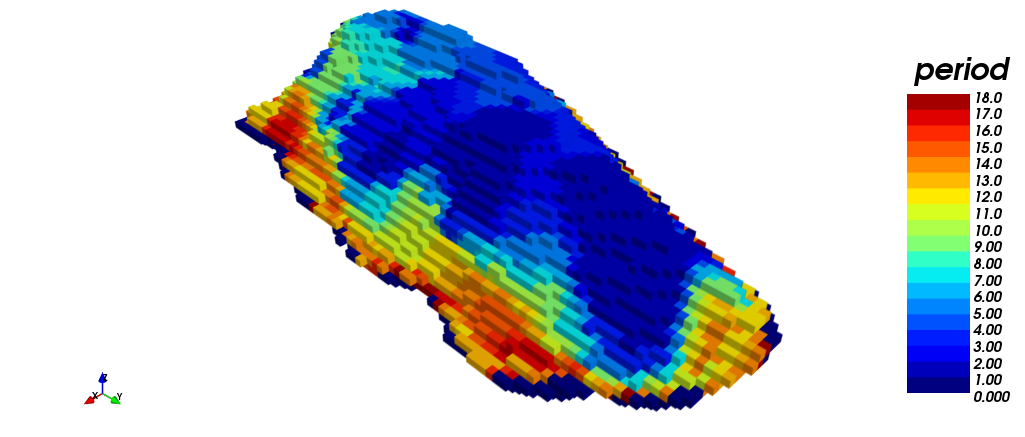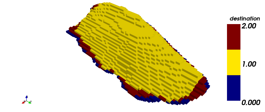(i)	(ii)
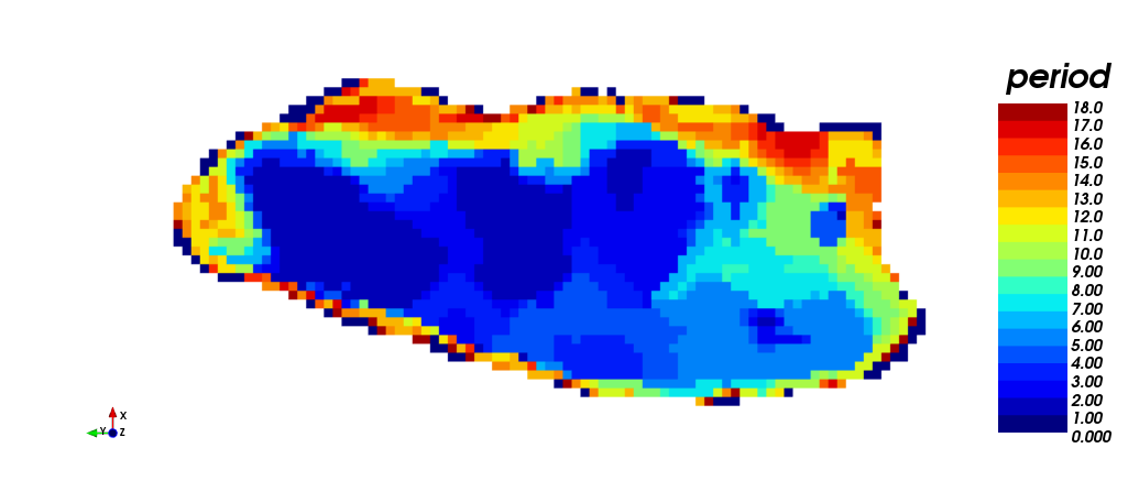(iii)	(iv)
(v)	(vi)

Production plan using toposort heuristic

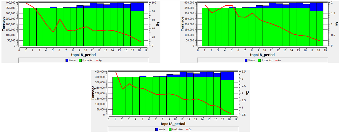
The production plan (mineral and waste) and the mean grade for each metal are shown in the following images.

 

Comparison and results

Considering the results obtained by both heuristics, it is clear that toposort made the schedule in 18 periods, as was required, meanwhile stw heuristic did the same in 17 periods. Looking at the production plans, topo could delayed the waste entrance in the first periods, classifying as mineral all the material extracyed between the periods 1 and 4, and also the 6th period, and from there extracting gradually the waste material completing the mine capacity in the final periods.
Meanwhile, STW made an homogeneous extraction, saturating both mine and plant capacities in most of the periods (except 16 and 17).
The myopic characteristic of STW doesnt let the heuristic to make decisions for later periods, instead of that, the heuristic make the best decisions possible for each period. On the other hand, topo is capable to make a global decision from the information obtained from the continuous solution of the original problem, and for this reasons is considered a robust decision, that is to say, to make a decision about a particular period, the heuristic looks what happen in later periods and then makes the decision.

In terms of cumulative present value (NPV), the topo strategy shows a greater NPV than the STW strategy (0.23% higher).

NPV STW : 1.386 [MUSD]

NPV TOPO : 1.390 [MUSD]

In general , this knd of strategies cannot ensure to find an optimal solution for the scheduling problem, but they are a good alternative considering real problems with great dimensions (number of blocks, periods and destinations), where the idea to solve directly is practicly