Below we present a number of illustrative examples of the use of MineLink through DOPPLER.
The objective of this article is to show generally the DOPPLER application and its features and to present illustrative examples of the use of some of the tools that it offers.
The main subjects to cover on this tutorial are the following:
- General view and layout.
- Creating a new project.
- Generating precedences.
- Generating new columnsl.
- Valuating blocks through DOPPLER.
- Calculating final pit.
- Calculating nested pits.
- Pit by Pit plot.
- Visualization tools.
- Using BOS2.
General view and layout.
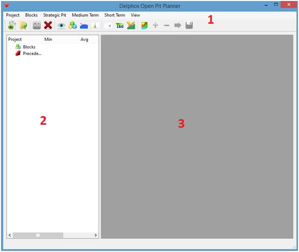
DOPPLER is an appliction that can be described in three parts. The first part is the one on the upper part of the window (1) which has an action menu and a toolbar. The second part is the project scheme panel on the left side of the window (2) on which the general characteristics of our project will be visible, such as the block model object ("Blocks" item) and the precedences sets ("Precedences" item). Also under this items will be some information about its components, for example at the "Blocks" item, a list of the block model columns as items will be visible. Finally, the third part is the right hand panel (3) which is essentially a mdi window on which every dialog and editing window will take place during the use of the application.
Creating a new project.
In order to create a new project on DOPPLER, the first step is to create a new project working folder somewhere in our computer. Once this folder has been created we need a text file with our block model data.
The block model file has to fullfill the following requirements:
- Regular. That is, every black has to have the same dimensions.
- First column: x-direction centriod.
- Second column: y-direction centriod.
- Third column: z-direction centriod.
- Fourth to n-th column: Attrinute columns definded by the user.
- The text file must be a tabulation or space separated file. Its extension must be ".txt".
- The first row is reserved for the names of the columns. The first three must be "x", "y" and "z" (lowercase). The rest of them are user defined.
- Data for blocks (except the names) must be numeric.
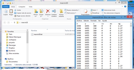
Below we give an example of such format:
x             y             z              cu           au           sg
3490      6495      300         0             0             2.27
3490      6495      330         0             0             2.27
3490      6495      360         0             0             2.27
3490      6495      390         0             0             2.27
3490      6495      420         0             0             2.27
3490      6495      450         0             0             2.27
The block model file can be placed anywhere but we reccomend you to put on the folder that you have created for the project.
Now we proceed in the following manner: Menu: Project->New:

Now a dialog window will appear on which it its aked to us to submit three paths. The forst one is the path to the block model file. The second one is the path to the (non existing yet) project file, the name of the file is user defined but its extension must be ".dp". We reccomend to place this file on the project folder (see the figure below). Finally the third path is for the project folder (the folder that we previously have created).
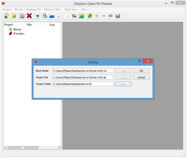
Now we press on the "Ok" button and we wait until the data from the block model is loaded into the application. If the importing was successfully we will be able to see the data of our block model on the left side panel under the "Blocks" item.
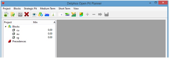
By pressing any field of the "Blocks" item we will be able to access the block model data on a table that will appear on the right side panel.
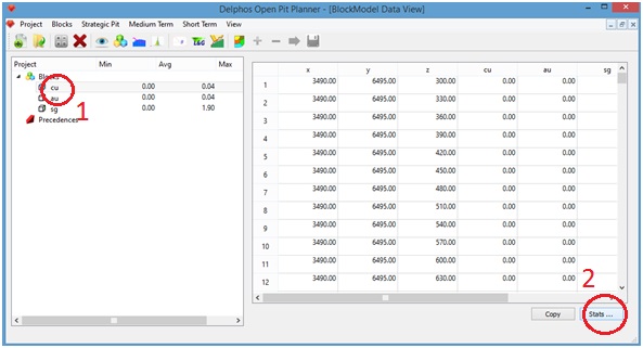
By pressing the "Stats" button (2) a window containing basic statistics of our block model will be presented.
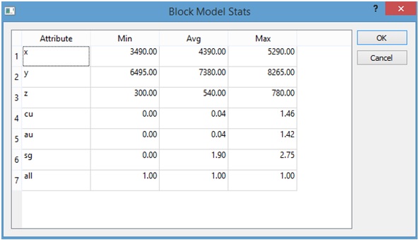
Generating precedences.
When we have a project created we can proceed to generate a set of precedence relationshiops between the blocks of our block model. MineLink allows the possibility of generate precedences by slope angle from a very general stand point: we can define for each block on the model an angular rose on the "xy" plane comprised by disjoint angular sectors that completes the whole circle (360° or 2pi rads). For each one of these sectors we define a different slope angle. The most simple case is the one on which we have the same slope angle for all the blocks in the model for all the directions on the "xy" plane. This is the case that we will be showing next.
As it was pointed on the previous paragraph, the precedences by slope can be constructed on a very general manner. That why for the simplest case we will need to create a dummy column on the block model that indicates that every block belongs to the same set. The idea is that every block on the has the same value on this column. This actually gives us a first glance to the way ion wich columns cab be added to the block model from DOPPLER.
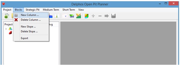
Menu: Blocks->New Column
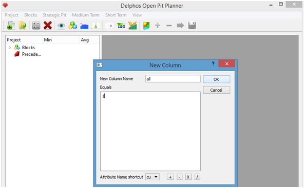
A dialog window will appear on which we must provide a name fro the neww column ("all" in our example, see below) and on the inferior box we can put the value for the column (as we can see on "Generating new columns" this box allow us to put functions that takes other existing columns of the block model as argument), in our case the value will be set on 1 (it could be any real number within ciomputing limiits). Then we press "Ok".
Now a new column named "all" should appear under the "Blocks" item. Next, Menu: Blocks->New Slope

A new dialog window will appear on which a name for the new precedence set, a value for the distance to consider for the construction of the arc cone, a name of an attribute of the block model (which indicates the blocks to consider), the value to search over this attribute and the angular sections to be considered are asked to us. As we stablished before, in our case we will submit the following data for the parameters:
- Z diff: 120 m (corresponds to 5 level relationship - 30*(5-1) -, because the size of the blocks on the z direction is 30 m).
- Block model attribute: all
- ID: 1
- Slope angle: 45 in all directions (360 -the whole circle- on "Valid for").
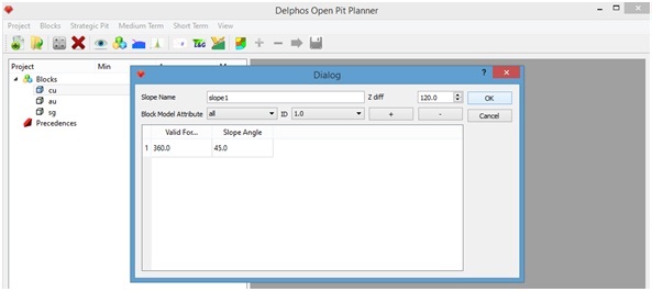
The "+" and "-" buttons allow us t add/remove angular sectors on the selection, The important thing is that sectors are defined as a valid partition of the [0,360] interval on the field "Valid for". As an example, if we are going to consider that every block on the sector comprised between 0° and 180° have a slope angle of 45° and those blocks between 180° and 270° have a slope angle of 50° and those between 270° and 360° have a slope angle of 60°, then on the first row of the table on "Vaid for" we must put a 180, and in "Slope Angle" a 45, on the second row we must put a 180 on the first field and a 50 on the second, and finally, on the third row we must put a 270 and a 60 respectively.
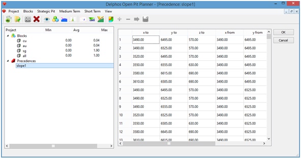
By pressing "Ok" the calculation of precedences takes place. When the process finishes we will be able to see a new precedence set under the "Precedences" item on the left side panel.
Generating new columns.
As it is shown on the "Generating precedences" section of this tutorial DOPPLER features the possibility of creating new columns on our block model. As a more elaborated example than the one shown on that section, we will generate a tonnage column to our block model from the existing "sg" column. We will assume that this column represent the volumetric density of each block on the model.
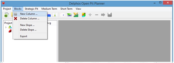
Menu: Blocks->New Column:
As our model has 30[m]x30[m]x30[m] dimensions for each block, we can enter the tonnage formula from the densty column "sg" like it is shown on the figure below.
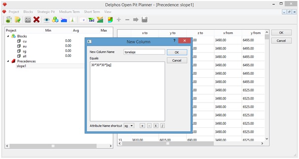
We press "Ok" and our new column must be visble from the left side panel, under the "Blocks" item with the submitted name on the dialog ("tonelaje" in our case).
Valuating blocks.
As it is shown on the "Generating precedences" and "Generating new column" sections, DOPPLER provides tools to generate new columns from already existing ones to the block model. This encourage us to think into perform a block valuation on a open pit mine site from DOPPLER.
Lets assume that we have the following values for the standard valuating parameters:
- Copper price: 2.5 [USD/lb Cu]
- Metallurgical recovery: 0.85 (en tanto por uno)
- Convesion factor: 2204.6 [lb/ton]
- Sell cost: 0.12 [USD/lb Cu]
- Mining cost: 1.6 [USD/t]
- Plant cost: 10 [USD/t]
- Blocks copper grade: [cu]
- Blocks tonnage: [tonelaje]
Here we are assuming that our block model has the columns of data ofr copper grade [cu] and tonnage [tonelaje].
Menu: Blocks->New Column:
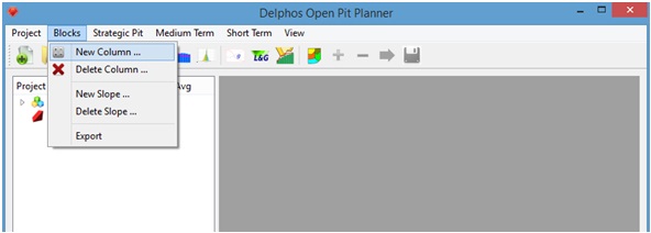
Using the usual formula for the calculation using the previously stated parameters, our equation look like:
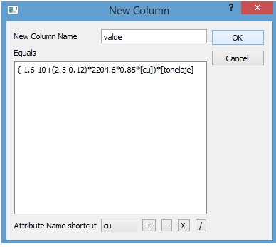
Notice that we have named "value" to our new column of values and that each time that we need to adress some of the existing columns in our block model we do so by putting its name between square brackets. So now we press the "Ok" button and when the process is done we will be able to see our new generated column con the left side panel under the "Blocks" item.
Calculating final pit.
In order to perform a final pit calculation we need a column in our block model that represents the actual mininig/processing value of each block. This column can be present on the block model from the begining or be created by the user (see, for instance the previous section). Also we need a set of precedences in our project (see "Generating precedences").
Assuming that we have those things (in our example the column "value" and the set "slope1", we can proceed in the following manner: Menu: Strategic Pit-> Final Pit
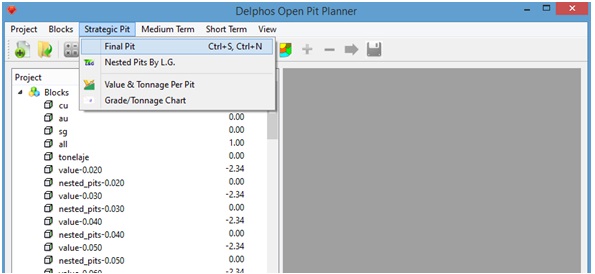
A dialog window will appear on which we must provide the name of value column, the set of precedences and the name of the binary attribute on which the solution will be stored on the block model (as a new column) the value 1 on this column means that the block belongs to the final pit (it is extracted) and the value 0 means that the block does not belong to the final pit (it is not extracted).
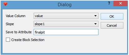
By pressing "Ok" the algorithm starts and at the end of it a new column with the stipulated name should be visible from the left side panel under the "Blocks" item.
Calculating nested pits.
DOPPLER also provides access to our MineLink implementation of the Lerchs $ Grossman algorithm from calculating nested pits. In order to use this algorithm we need a set of precedences previously created in our DOPPLER project (see "Generating precedences"). Given all that, we proceed as it follows: Menu: Strategic Pit-> Nested Pits by L.G.
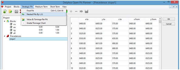
A new dialog window will appear on wich we must provide information about the instance parameters to be used. For our example we will use the following values:
- Copper price: 1.7 [USD/lb Cu]
- Metallurgical recovery: 0.85
- Conversion factor: 2204.6 [lb/t]
- Sell cost: 0.12 [USD/lb Cu]
- Mining cost: 1.6 [USD/t]
- Plant cost: 10 [USD/t]
- Copper grade: cu
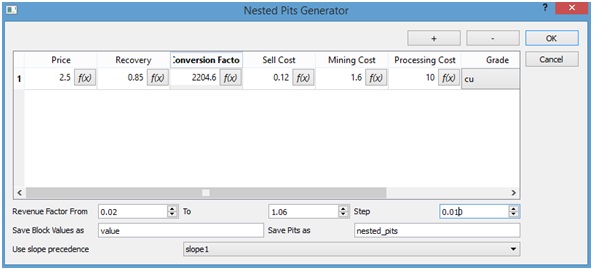
As it an be seen at the previous figure, the revenue factor is entered as an interval ("From", "To") and with a step ("Step"). The idea is to calculate the first pit with the "From" value and then generate the next value adding "Step" to the previous ravenue factor an so on until we recah the "To" value. Also we need to enter a name-prefix to the new columns that are going to be added to the block model with the correponding value associated with the successive revenue factors ("Save Block Values as"), a name-prefix for the resulting pit solutions (see "Calculating final pit") columns it is asked too ("Save Pits as"). Finally we must select a previously generated set of precedences to be used (see "Generating precedences"). Moreover it can be seen from the figure that each cell of the table has a button ("f(x)") this button allows to enter a fomula (see "Generating new columns " and "Valuing blocks") for the cell instead of a fixed value. By pressing the "Ok" button a progress bar will appear on the screen.
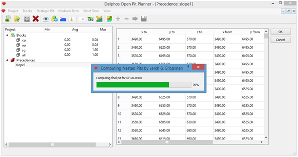
At the end of the process all the newly generated columns will be visible at the left side panel, under the "Blocks" item.

As it is shown above, the names generated for both, values and pit columns are in the format: prefix-RFValue.
Pit by Pit plot.
A graphic tool of great help for analysing the result of a nested pits solution (see last section) is the Pit by Pit plot. Which shows for each resulting pit (by revenue factor) the total tonnage and the resulting total value fro the pit.
Menu: Strategic Pit-> Value & Tonnage per Pit
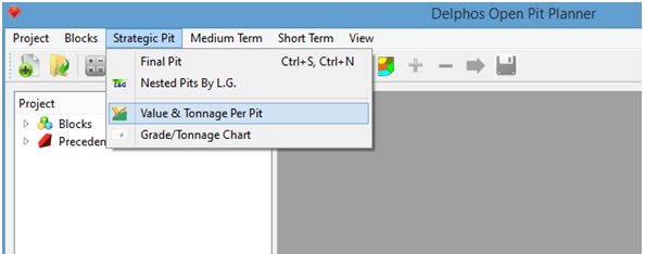
A dialog window will appear on which we are asked to enter, respectively, the name-prefix of the solution columns, the name-prefix for the value columns and the name of the tonnage column in the block model. If we use the data from the last section we need to enter the data as it is shown in the figure below:
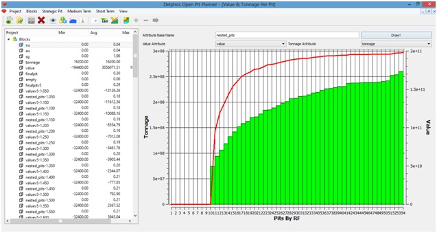
Onece the data is entered we click on the "Draw!" button and we will get a plot like the one that is shown on the previous figure.
Visualization tools.
DOPPLER provides two visualization tools for block model data. The first one is block visualization according some columns on the block model.
Menu: View->Blocks
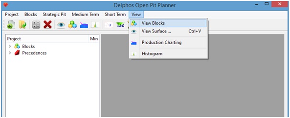
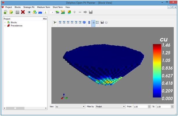
A new window will be docked onto the right side panel. For exmaple purposes we will assume that we have two columns in the block model. The first one is a binary column named "finalpit" which represent if a block is extracted (1) or not (0), the second one is a column named "cu" wich represent the blocks copper grade.
In order to be able to visualize the blocks we must decide:
- The column from which the blocks wil be selected: finalpit
- The column with the values that we want to see on the blocks: cu
- The range of values from the selection : "From" 1.0 "To" 1.0
This options re entered at the bottom of the docked window see the figure below.
The data that we have selected means that we are going to see all the extracted blocks and these will be painted accordingly to their grade value.
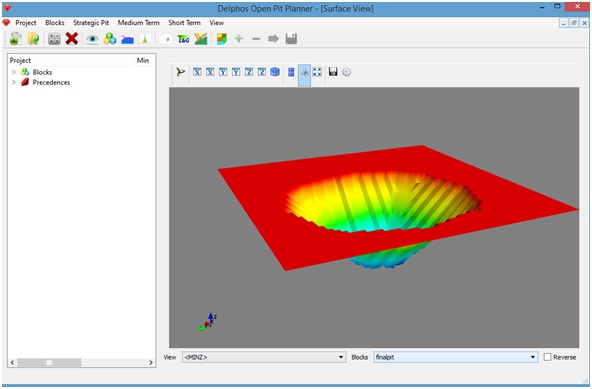
The second option is surface visualization.
Menu: View->View Surface

A new window will be docked at the right side panel.
In order to visualize the data we must select if we want to see the upper part of the selection or the lower part. In this example we are going to select the lower part:
- View: <MINZ>
This visualization tool requires a binary column at the block model in order to indentify the set of blocks. Both parameters are entered at the bottom of the docked window.
Using BOS2
DOPPLER provides a module that alows to use BOS2. In order to use this module we only need a block model with the appropiate columns on it. In order to follow this tutorial we reccomend a previous reading of all other sections of this article.
Let us consider the following illustrative mine scheduling problem. We have two destinations, plant and waste; and two preexisting stocks. The block model has the value columns for each destinationand we know the value per destination from the stocks. We want to schedule to a 3 period horizon considering transport constraints on both destinations and blending constriants on a contaminat for the plant.
We start from a previosly loaded block model onto DOPPLER that has 4 columns and a previosly created set of precedences as it is shown in the next figure.
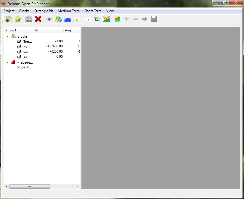
In order to use the BOS2 module we proceed as follows:
Menu: Short Term-> Short Term Scheduler.
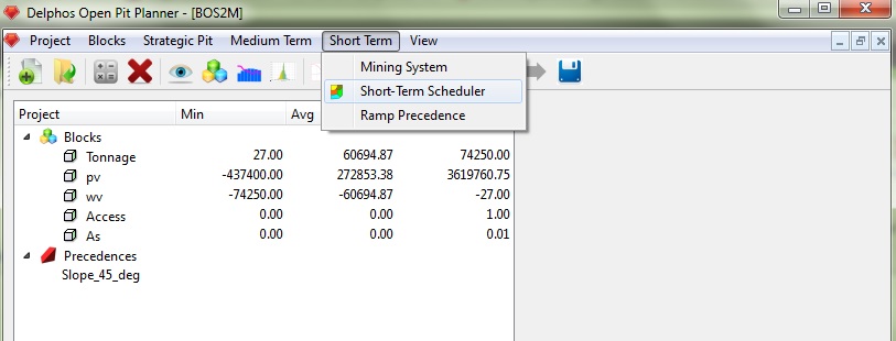
A new working window will be docked at the right side panel.
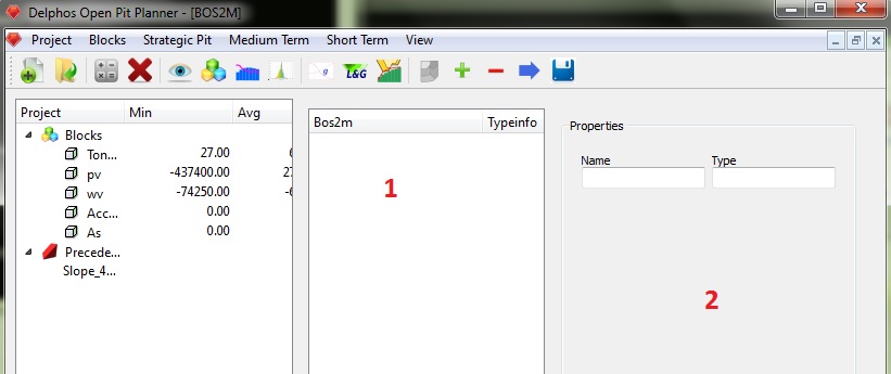
At the previous figure we can see that the window is comprised of two ne panels. The first one (1), wich we are going to refer as the scheme panel, is where we are going to see a tree-node scheme of our BOS2 instance, and the second one (2) is the properties editing panel which all the parameters values will be set for each node of our instance.
In order to begin we must first create a root node, which will always be a Scheduling Instance type node. To add/remove nodes from our instance we will make use of the "+" and "-" buttons on the toolbar. One important thing to consider is that the atual option that we will get for adding nodes depend on the current selection node on the scheme panel (1), when there is no current selection active only the defaul option will be presented (Scheduling Instance node).
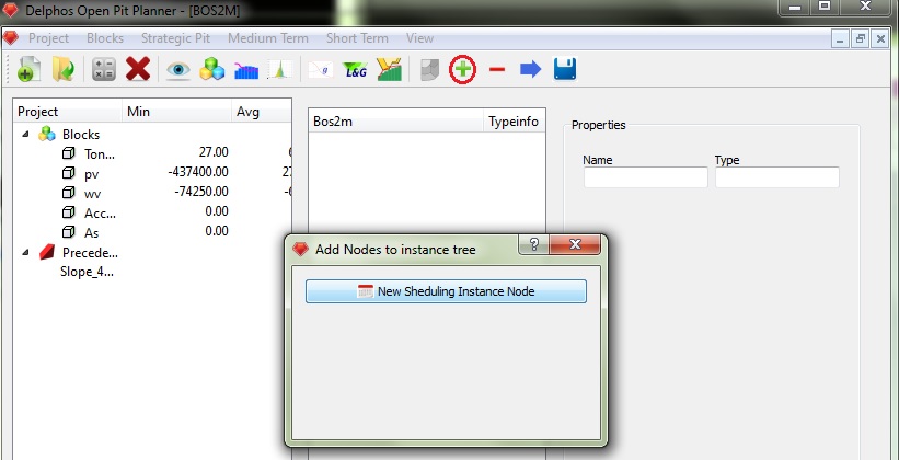
In the previous figure we show the dialog window that appears when the "+" is clicked on the toolbar. In this case, because the instance is empty, We will only see the "New Scheduling Instance Node" option. By pressing this button a number of node will be added to our scheme panel.
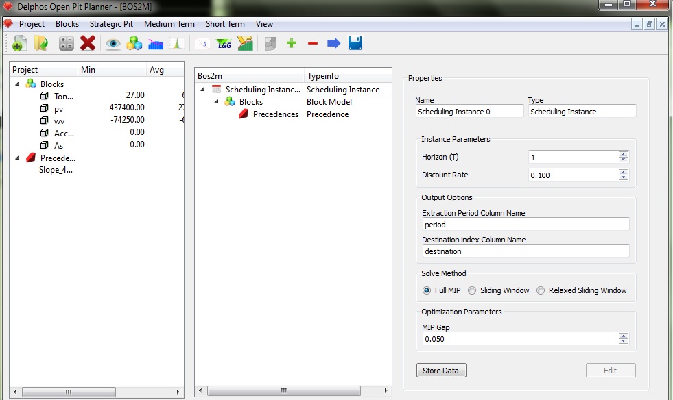
In the previous figure we can see the nodes that are added. A root node ("Scheduling Instance" type node), and in addition a "Blocks" node (which represent the block model) and a "Precedences" node (wich represent the set of precedences). Also we can see that the current selection on the scheme panel is the root node, that why we see at the properties panel the editing options for this node. This also occurs with all the other types of nodes.
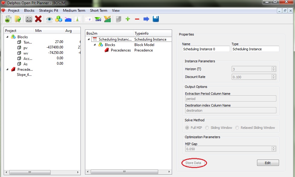
On the properties panel, all the nodes has an user editable name for the node and non editable type of the node. Fro example purposes, we will always leave the default name for the nodes as we move on. As we stablished before we want to schedule over 3 periods ("Horizon"), we are going to use a discount rate of 10% (Discount Rate). Also we want the resulting schedule to be stored as columns in the block model so we need to enter the names for those columns ("Extraction period Column Name" and "Destination Column Name"). Next we need to select the solution method for our problem, which we set on "Full MIP" (this means we are going to ask for the full MIP solution to our problem, the other options are heuristic-based approachs to the full MIP model). Next we need to set the MIP GAP for the Branch and Cut algorithm (this is a delicate subject and needs prior knowledge on Integer Programming). So wen all the data has been entered we must save it by clicking on the "Store Data" button. By doing so all the editing fields becomes unactive and if we want to edit something we must clivk on the "Edit" button change whatever we want and the click on the "Store Data" again. This is most important because as we move on the construction of the BOS2 instance, the module always ask us to save our progress in order to keep moving on. It it good to mention that all the editing windows for all the nodes follows the same idea, thats why they all have this two buttons on the same exact position (with different names in some ocasions).
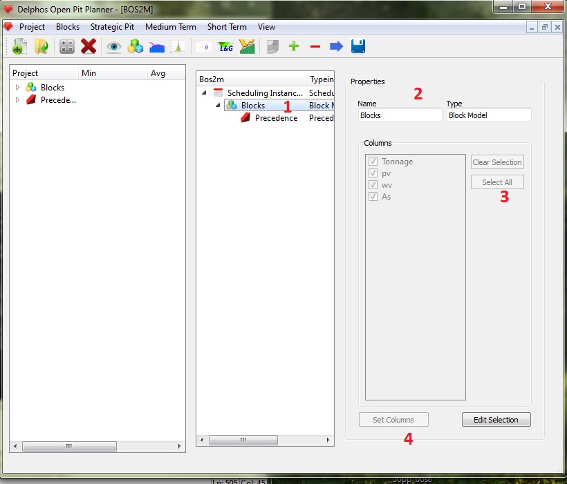
The next step will be select the columns of the block model that will be used by the module. So we first click on the "Blocks" node (1). The properties window will update to a block model properties window. We leave the default name on the properties window (2) and then we select our desired columns from the list inside the lower box. As we want to use all the columns in the model (at least in this example we want to do so) we click on the "Select All" button (4) and then we store our data (4). This step is very important because all the following properties windows for any child node will only see the selected columns.
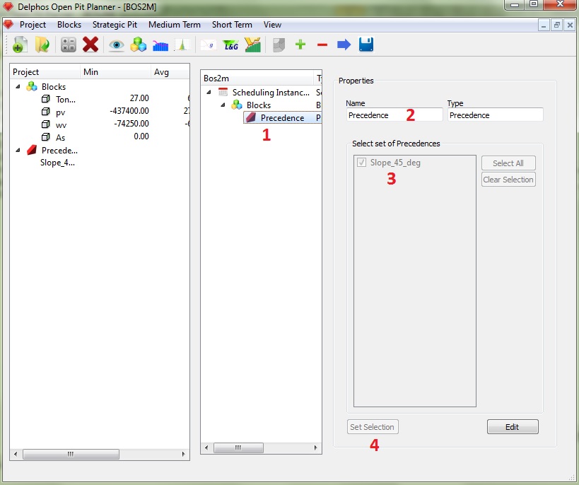
In the previous figure it is shown how to select the precedence sets that are going to be used in our instance. First we click on the "Precedence" node on the scheme panel (1) then we can give a new name for the node (2) and then we can select one or more precedence sets from the list inside the lower box (3). Once we have selected our set(s) we save our data (4) and we can move on. It its good to mention that the list that is shown on the box will only show the sets of precedences that already exist when the module was started.
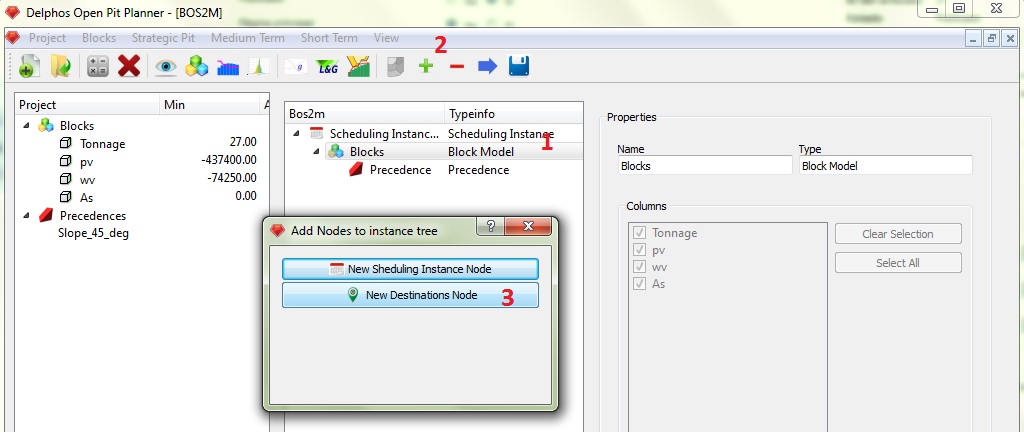
The next step is to generate destinations for our instance. As the destinations requiere information from the block model, then the destinations nodes are always child nodes from a block model node. Click on the "Blocks" node (1), click on the "+" button on the toolbar (2) then select "New Destinations Node" from the dialog (3).
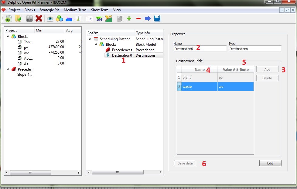
In the previous figure we can see the added destinations node. In order to actually create our instance destinations (plant and waste) we proceed as follows. First we click on the newly created node (1) and we choose a name for it if we want to do so (2). Then for crating our destinations we must click on the "Add" button (2) a number of times equal to the desired number of destinations (two in our case). Each time we click on this button a new row will be appended to the destinations table. This table has two fields, "Name" (on which we can name as we want our destinations) and "Value Attribute" (on which we need to privide of an existing column of the block model that represents the value column for the current destination). In order to edit the cells on the table (and the process is the same for all the remaining tables on the module) we must click once on the desired cell and and editor will appear inside it. This editor will vary according the nature of the field, sometimes a linedit will appear (text), sometimes a combobox will (closed selection), sometimes a spinbox will (numeric) and in other times a checkbox will (binary). In this case Clearly the "Name" field is text and the "Value Attribute" field is closed selection (from the list of columns selected on the block model node). Finally we save our data (6).
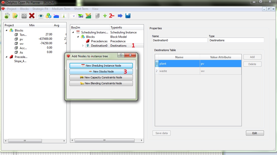
The next step will be creating our preexisting stocks. As stocks needs information of the value attributes of the destinations, they are always going to be child nodes of destinations nodes. So, we first click on the destinations node (1) then we click on the "+" button on the toolbar (2). The dialog will appear and we select "Add Stock Node" (3). The new stock node will be placed under the selected destinations node.
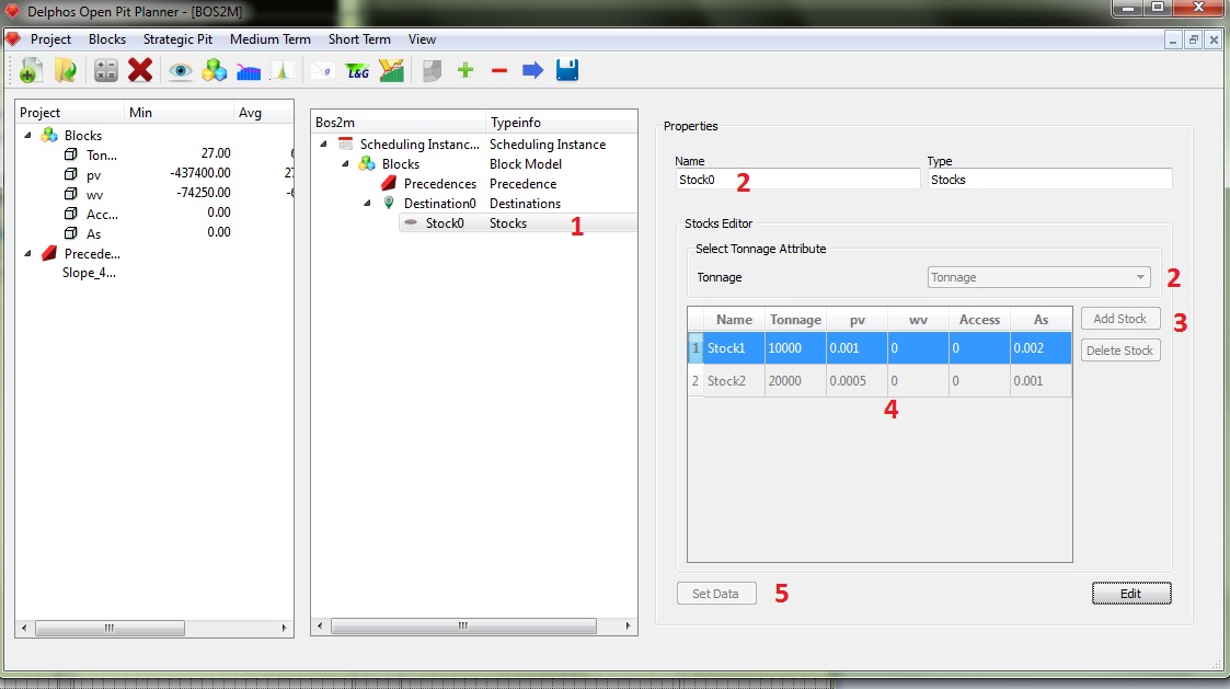
In order to actually create our stocks, we first click on the stocks node (1), and we name our new node if we want to (2). Next we need to select the column on the block model that represents the tonnage for the blocks (we need one, always) (3). Then we create the stocks on a similar way on which we create destinations, by using the "Add Stock" button (4). The we edit the fields on the table (5). The fields on the stocks table are "Name", "Tonnage" (initial tonnage for the stock), and the others correspond to the selected block model columns and must have value.
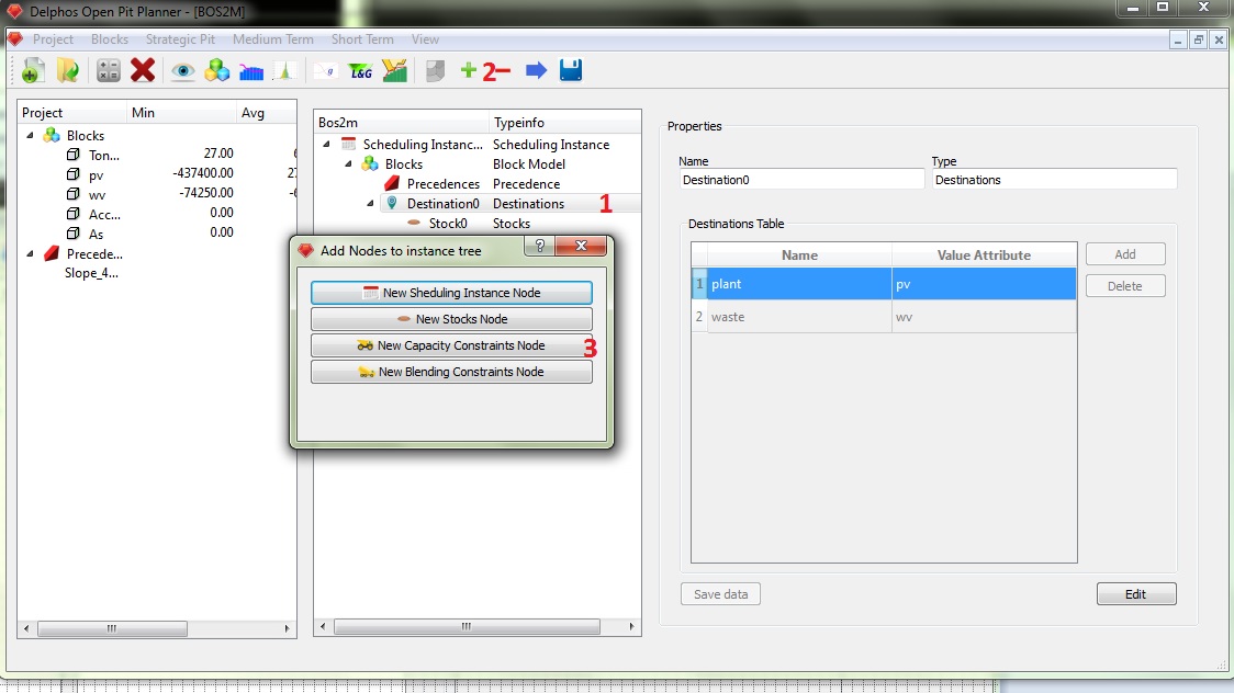
Now we need add our transportation constraints into our instance. The capacity constrints need information from the a destinations node so they are going to be always a child node from a destination node. We select the destination node (1), we click on the "+" button on the toolbar (2) and we select "Add Capacity Constraints Node" from the dialog (3). The new node will be placed under the selected destination node.
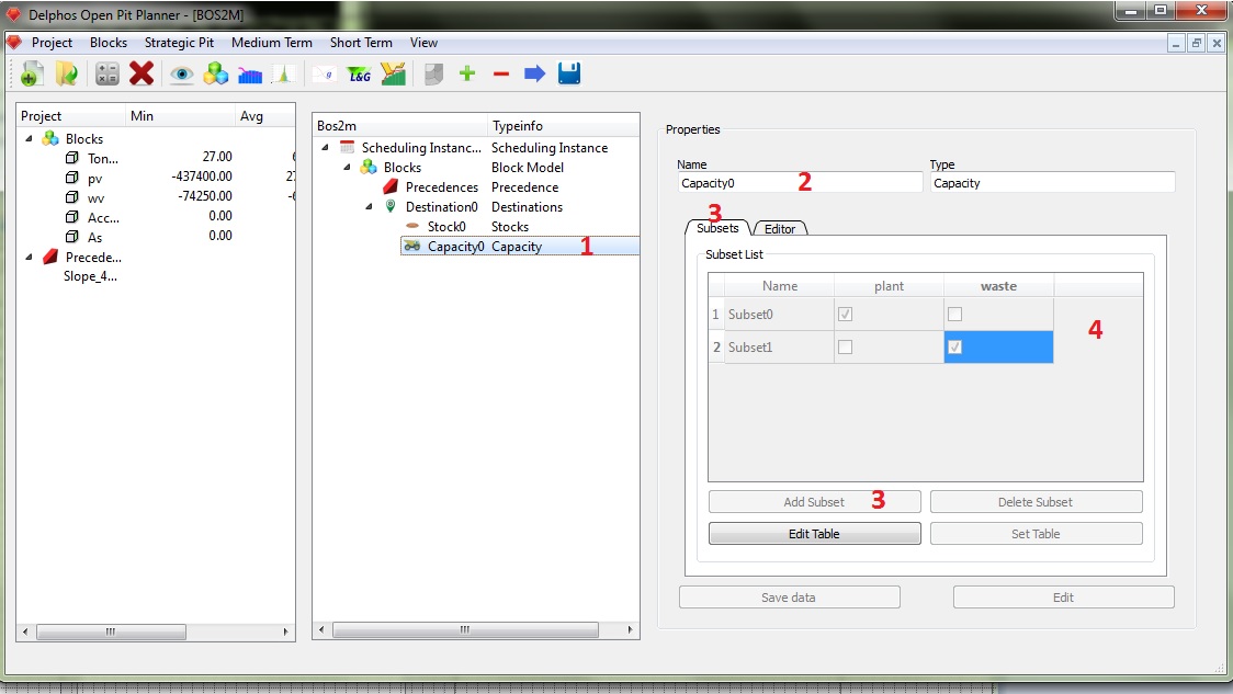
In order to create our transportation constraints we must proceed as it follows. we click on the capacity node (1), we can name it if we want to (2). Select the "Subset" tab (3). This tab alow us to create any subset from the set of destinations (the one we create at the corresponding destinations node). This subsets are used on the constraints, because a constraint can be active on any number of destinations (in our case we could want a "total" transport constraint wich involves both destinations). In our example que decided that the constraints will operate on each destination separately, that why we need to create two subsets using the "Add Subset" button (4), the we select the destinations that comprise each subset (4) and we set our data ("Set Table").
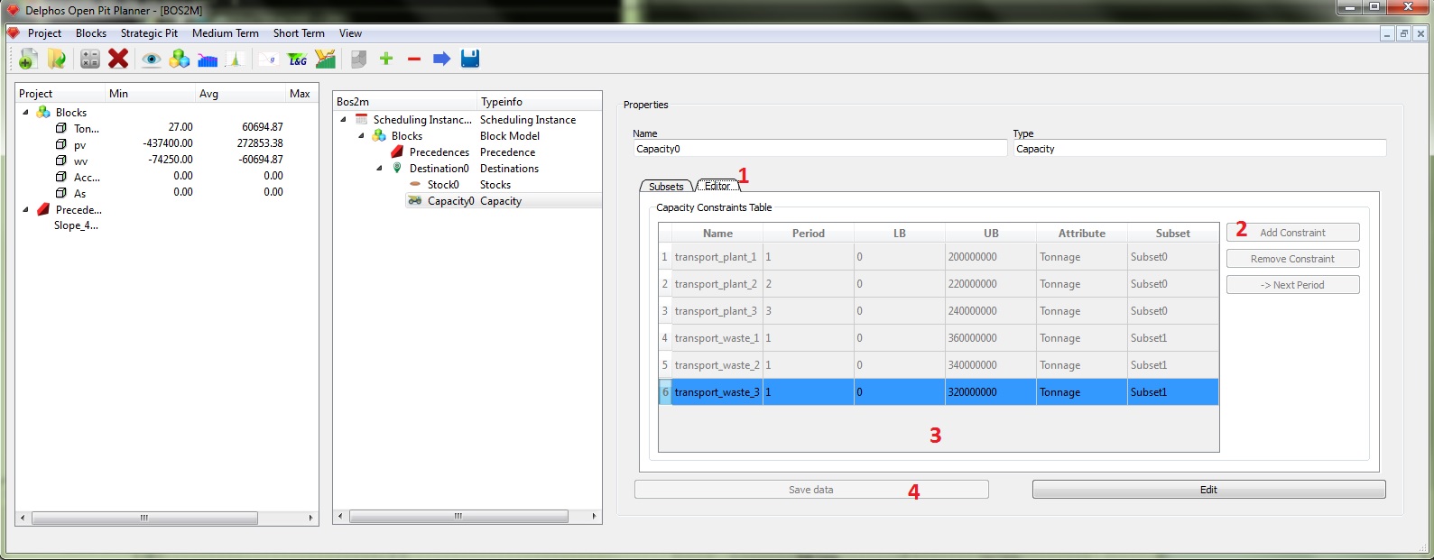
Now we can move on to the next tab. Click on the "Editor" tab (1) y we add the amount of desired constraints using the "Add Constraint" button (2). As every constraint is bounded to a specific period, and we have 3 periods and we want to constrain both the plan and waste separately we are going to need 6 constraints. Click the "Add Constraint" six times and edit the fields on the table. the first field is "Name" (its important that the names entered be different for each row), the second "Period" indicates the period on wich the constraint will be placed, the third and fourth "LB" and "UB" indicates the minimum and maximum values to be used for the amount sended to the corresponding subset, the fifth "Attribute" indicates the column of the block model that is to be added and finally "Subset" indicates which of the previously created subsets (at the previous tab) is going to be used. When all the data is entered on the table (3), then we can save our data (4) .
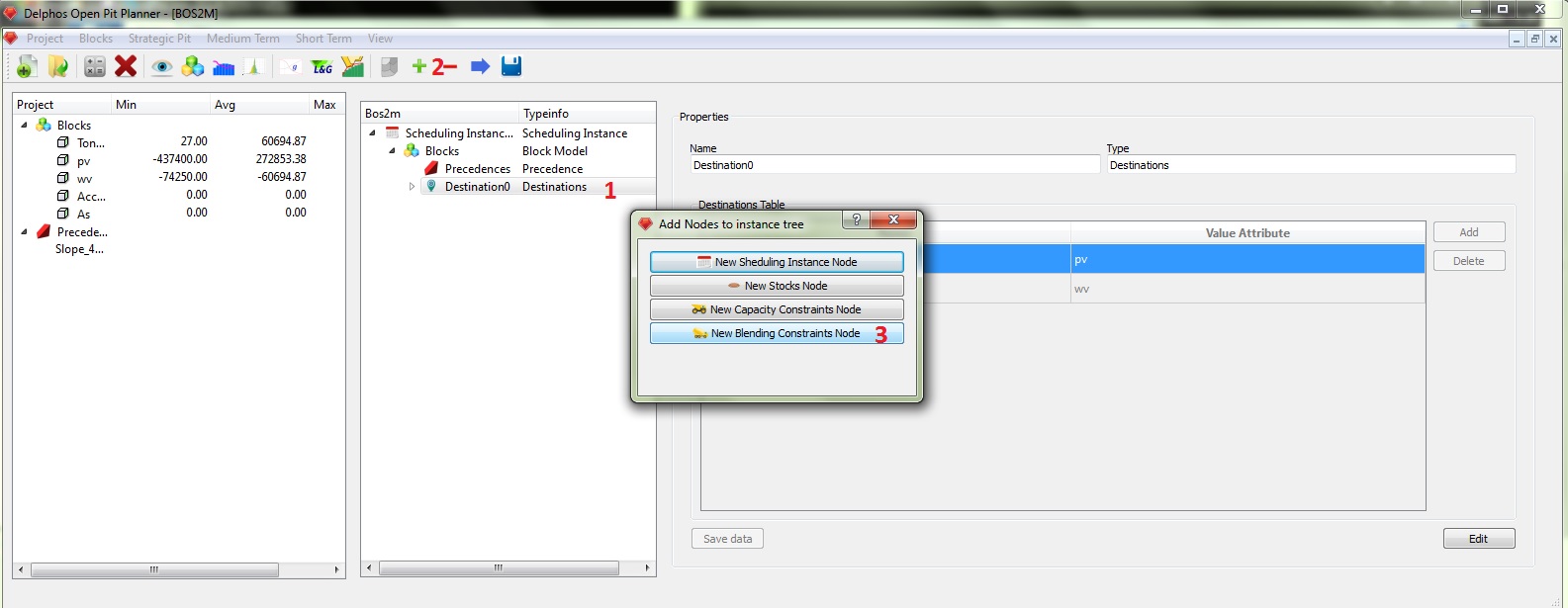
So now its turn of the blending constraints. In our block model we have a column named "As" that represent the concentration (percentage) of arsenic on each block. So we are interested on constrain (upper bound) the mean amount of arsenic that goes to the plant on each period.
Just like the capacity node a blending node depends on the information on the destination nodes, so it will be always a child node from a destination node.
Select the destination node (1), then press the "+" button on the toolbar (2) and then select "New Blending Constraints Node" from the dialog window (3).
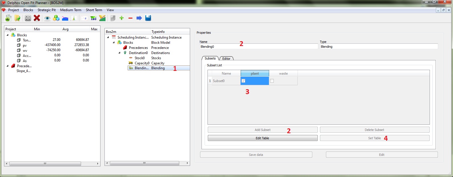
The scheme for creating blending constraints is completly analogous to the capacity constraints. The only difference is that we have an extra field on the constraints table.
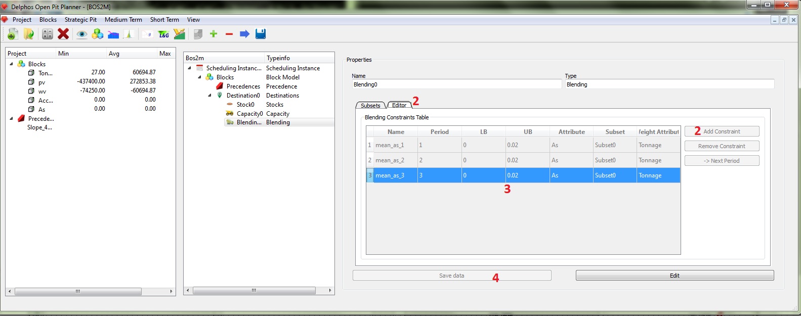
In the blending constraints table we have a new field "Weight Attribute" which represents the weight on the weighted average on every period calculation. I our exmaple we want to constrains the mean percentage of arsecnic that gooes to the plant on every period, so we need three constraints. In the previous figure we can see an example for the blending constraints data. And as its usual we save our data to finish. With this we have created our instance.
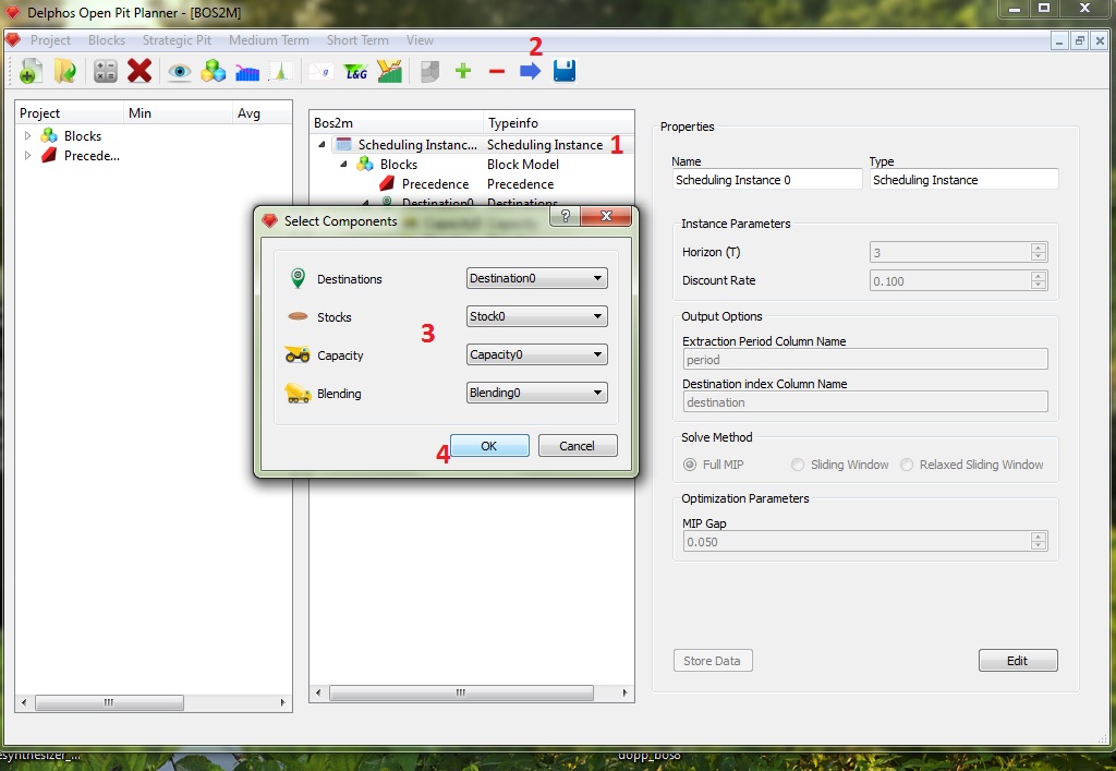
Now we are ready to solve our instance. Click on oyur root node (1) then click on the blue arrow on the toolbar (2). A "Select Components" dialog will appear. In this dialog we must select each component of our instance (this is due to the fact that we can have, for example multiple destinations nodes as childs of the same block model node). So we select the names of our nodes (3) and click "Ok" (4).
At that moment the optimization process takes place. Process that can be extremly time consuming depending on the size of the block model, the constraints, the parameter values and mostly the solution method selected. During the optimization process the application becomes inactive and it comes back only when a solution has been found (or not, depending on the results of the solver).
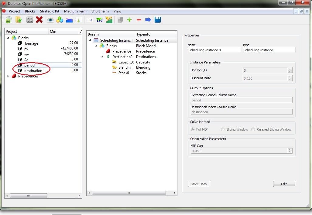
When the process finishes, we should be able to see the new solution columns on the block model as it is shown on the previous figure. From here on, any analisys or visualization tool can be performed from DOPPLER.


